4. Automatic Program Optimization
4.1. Prelude
In the past chapters, we learned about how to build primitive tensor functions and connect them to form end-to-end model executions. There are three primary types of abstractions we have used so far.
A computational graph view that drives the high-level executions.
Abstraction for primitive tensor functions.
Library function calls via environment function registration.
All of these elements are encapsulated in an IRModule. Most of the MLC processes can be viewed as transformations among tensor functions.
There are many different ways to transform the same program. This chapter will discuss ways to automate some of the processes.
4.2. Preparations
To begin with, we will import necessary dependencies and create helper functions.
import numpy as np
import tvm
from tvm import relax
from tvm.ir.module import IRModule
from tvm.script import relax as R
from tvm.script import tir as T
import IPython


def code2html(code):
    """Helper function to use pygments to turn the code string into highlighted html."""
    import pygments
    from pygments.formatters import HtmlFormatter
    from pygments.lexers import Python3Lexer
    formatter = HtmlFormatter()
    html = pygments.highlight(code, Python3Lexer(), formatter)
    return "<style>%s</style>%s\n" % (formatter.get_style_defs(".highlight"), html)
4.3. Recap: Transform a Primitive Tensor Function.
Let us begin by reviewing what we did in our previous chapters – transforming a single primitive tensor function.
@tvm.script.ir_module
class MyModule:
    @T.prim_func
    def main(
        A: T.Buffer((128, 128), "float32"),
        B: T.Buffer((128, 128), "float32"),
        C: T.Buffer((128, 128), "float32"),
    ):
        T.func_attr({"global_symbol": "main", "tir.noalias": True})
        for i, j, k in T.grid(128, 128, 128):
            with T.block("C"):
                vi, vj, vk = T.axis.remap("SSR", [i, j, k])
                with T.init():
                    C[vi, vj] = 0.0
                C[vi, vj] = C[vi, vj] + A[vi, vk] * B[vk, vj]
First, let us define a set of inputs and outputs for evaluation.
dtype = "float32"
a_np = np.random.rand(128, 128).astype(dtype)
b_np = np.random.rand(128, 128).astype(dtype)
c_mm = a_np @ b_np
We can build and run MyModule as follows.
a_nd = tvm.nd.array(a_np)
b_nd = tvm.nd.array(b_np)
c_nd = tvm.nd.empty((128, 128), dtype="float32")

lib = tvm.build(MyModule, target="llvm")
f_timer_before = lib.time_evaluator("main", tvm.cpu())
print("Time cost of MyModule: %.3f ms" % (f_timer_before(a_nd, b_nd, c_nd).mean * 1000))
Time cost of MyModule: 3.150 ms
Next, we transform MyModule a bit by reorganizing the loop access
pattern.
def schedule_mm(sch: tvm.tir.Schedule, jfactor=4):
    block_C = sch.get_block("C", "main")
    i, j, k = sch.get_loops(block=block_C)
    j_0, j_1 = sch.split(loop=j, factors=[None, jfactor])
    sch.reorder(i, j_0, k, j_1)
    sch.decompose_reduction(block_C, k)
    return sch
sch = tvm.tir.Schedule(MyModule)
sch = schedule_mm(sch)
IPython.display.HTML(code2html(sch.mod.script()))
# from tvm.script import ir as I
# from tvm.script import tir as T

@I.ir_module
class Module:
    @T.prim_func
    def main(A: T.Buffer((128, 128), "float32"), B: T.Buffer((128, 128), "float32"), C: T.Buffer((128, 128), "float32")):
        T.func_attr({"tir.noalias": T.bool(True)})
        # with T.block("root"):
        for i, j_0 in T.grid(128, 32):
            for j_1_init in range(4):
                with T.block("C_init"):
                    vi = T.axis.spatial(128, i)
                    vj = T.axis.spatial(128, j_0 * 4 + j_1_init)
                    T.reads()
                    T.writes(C[vi, vj])
                    C[vi, vj] = T.float32(0.0)
            for k, j_1 in T.grid(128, 4):
                with T.block("C_update"):
                    vi = T.axis.spatial(128, i)
                    vj = T.axis.spatial(128, j_0 * 4 + j_1)
                    vk = T.axis.reduce(128, k)
                    T.reads(C[vi, vj], A[vi, vk], B[vk, vj])
                    T.writes(C[vi, vj])
                    C[vi, vj] = C[vi, vj] + A[vi, vk] * B[vk, vj]
Then we can build and run the re-organized program.
lib = tvm.build(sch.mod, target="llvm")
f_timer_after = lib.time_evaluator("main", tvm.cpu())
print("Time cost of MyModule=>schedule_mm: %.3f ms" % (f_timer_after(a_nd, b_nd, c_nd).mean * 1000))
Time cost of MyModule=>schedule_mm: 0.699 ms
4.3.1. Transformation Trace
Besides sch.mod field, another thing tir.Schedule offers is a
trace field that can be used to show the steps involved to get to the
transformed module. We can print it out using the following code.
print(sch.trace)
# from tvm import tir
def apply_trace(sch: tir.Schedule) -> None:
  b0 = sch.get_block(name="C", func_name="main")
  l1, l2, l3 = sch.get_loops(block=b0)
  l4, l5 = sch.split(loop=l2, factors=[None, 4], preserve_unit_iters=True, disable_predication=False)
  sch.reorder(l1, l4, l3, l5)
  b6 = sch.decompose_reduction(block=b0, loop=l3)
def schedule_mm(sch: tvm.tir.Schedule, jfactor=4):
    block_C = sch.get_block("C", "main")
    i, j, k = sch.get_loops(block=block_C)
    j_0, j_1 = sch.split(loop=j, factors=[None, jfactor])
    sch.reorder(i, j_0, k, j_1)
    sch.decompose_reduction(block_C, k)
    return sch
The above trace aligns with the transformations we specified in
schedule_mm. One thing to note is that the trace (plus the original
program) gives us a way to completely re-derive the final output
program. Let us keep that in mind; we will use trace throughout this
chapter as another way to inspect the transformations.
4.4. Stochastic Schedule Transformation
Up until now, we have specified every detail about what transformations we want to make on the original TensorIR program. Many of those choices are based on our understanding of the underlying environment, such as cache and hardware unit.
However, in practice, we may not be able to decide every detail accurately. Instead of doing so, we would like to specify what are possible ways to transform the program, while leaving out some details.
One natural way to achieve the goal is to add some stochastic (randomness) elements to our transformations. The following code does that.
def stochastic_schedule_mm(sch: tvm.tir.Schedule):
    block_C = sch.get_block("C", "main")
    i, j, k = sch.get_loops(block=block_C)
    j_factors = sch.sample_perfect_tile(loop=j, n=2)
    j_0, j_1 = sch.split(loop=j, factors=j_factors)
    sch.reorder(i, j_0, k, j_1)
    sch.decompose_reduction(block_C, k)
    return sch
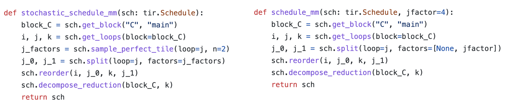
Let us compare stochastic_schedule_mm and schedule_mm side by
side. We can find that the only difference is how to specify
j_factors. In the case of schedule_mm, j_factors is passed
in as a parameter specified by us. In the case of
stochastic_schedule_mm, it comes from sch.sample_perfect_tile.
As the name suggests, sch.sample_perfect_tile tries to draw random
numbers to fill in j_factors. It samples factors such that they
perfectly split the loop. For example, when the original loop size is
128, possible ways to split the loop include: [8, 16],
[32, 4], [2, 64] (note 8 * 16 = 32 * 4 = 2 * 64 = 128).
Let us first try to see what is the effect of stochastic_schedule_mm
by running the following code-block. Try to run the following code block
multiple times and observe the outcome difference. You might find that
the loop bound of j_1 changes each time we run the code-block.
sch = tvm.tir.Schedule(MyModule)
sch = stochastic_schedule_mm(sch)

IPython.display.HTML(code2html(sch.mod.script()))
# from tvm.script import ir as I
# from tvm.script import tir as T

@I.ir_module
class Module:
    @T.prim_func
    def main(A: T.Buffer((128, 128), "float32"), B: T.Buffer((128, 128), "float32"), C: T.Buffer((128, 128), "float32")):
        T.func_attr({"tir.noalias": T.bool(True)})
        # with T.block("root"):
        for i, j_0 in T.grid(128, 16):
            for j_1_init in range(8):
                with T.block("C_init"):
                    vi = T.axis.spatial(128, i)
                    vj = T.axis.spatial(128, j_0 * 8 + j_1_init)
                    T.reads()
                    T.writes(C[vi, vj])
                    C[vi, vj] = T.float32(0.0)
            for k, j_1 in T.grid(128, 8):
                with T.block("C_update"):
                    vi = T.axis.spatial(128, i)
                    vj = T.axis.spatial(128, j_0 * 8 + j_1)
                    vk = T.axis.reduce(128, k)
                    T.reads(C[vi, vj], A[vi, vk], B[vk, vj])
                    T.writes(C[vi, vj])
                    C[vi, vj] = C[vi, vj] + A[vi, vk] * B[vk, vj]
What is happening here is that each time we run
stochastic_schedule_mm it draws a different j_factors randomly.
We can print out the trace of the latest one to see the decisions we
made in sampling.
print(sch.trace)
# from tvm import tir
def apply_trace(sch: tir.Schedule) -> None:
  b0 = sch.get_block(name="C", func_name="main")
  l1, l2, l3 = sch.get_loops(block=b0)
  v4, v5 = sch.sample_perfect_tile(loop=l2, n=2, max_innermost_factor=16, decision=[16, 8])
  l6, l7 = sch.split(loop=l2, factors=[v4, v5], preserve_unit_iters=True, disable_predication=False)
  sch.reorder(l1, l6, l3, l7)
  b8 = sch.decompose_reduction(block=b0, loop=l3)
When we look at the trace, pay close attention to the decision=[...]
part of sample_perfect_tile. They correspond to the value that the
sampling_perfect_tile picked in our last call to
stochastic_schedule_mm.
As an alternative way to look at different samples of
stochastic_schedule_mm, we can run the following block multiple
times and look at the trace.
sch = tvm.tir.Schedule(MyModule)
sch = stochastic_schedule_mm(sch)
print(sch.trace)
# from tvm import tir
def apply_trace(sch: tir.Schedule) -> None:
  b0 = sch.get_block(name="C", func_name="main")
  l1, l2, l3 = sch.get_loops(block=b0)
  v4, v5 = sch.sample_perfect_tile(loop=l2, n=2, max_innermost_factor=16, decision=[32, 4])
  l6, l7 = sch.split(loop=l2, factors=[v4, v5], preserve_unit_iters=True, disable_predication=False)
  sch.reorder(l1, l6, l3, l7)
  b8 = sch.decompose_reduction(block=b0, loop=l3)
4.4.1. Deep Dive into Stochastic Transformation
Now let us take a deeper dive into what happened in stochastic schedule transformations. We can find that it is a simple generalization of the original deterministic transformations, with two additional elements:
Random variables that come from
sample_perfect_tileand other sampling operations that we did not cover in the example.Schedule operations that take action depending on the random variables.
Let us try to run the stochastic transformation step by step.
sch = tvm.tir.Schedule(MyModule)
block_C = sch.get_block("C", "main")
i, j, k = sch.get_loops(block=block_C)
j_factors = sch.sample_perfect_tile(loop=j, n=2)
type(j_factors[0])
tvm.tir.expr.Var
Elements in the j_factors are not real integer numbers. Instead,
they are symbolic variables that refer to a random variable being
sampled. We can pass these variables to the transformation API to
specify choices such as factor values.
print(sch.trace)
# from tvm import tir
def apply_trace(sch: tir.Schedule) -> None:
  b0 = sch.get_block(name="C", func_name="main")
  l1, l2, l3 = sch.get_loops(block=b0)
  v4, v5 = sch.sample_perfect_tile(loop=l2, n=2, max_innermost_factor=16, decision=[128, 1])
The schedule trace keeps track of the choices of these symbolic
variables in the decisions field. So follow-up steps will be able to
look up these choices to decide how to split the loop.
IPython.display.HTML(code2html(sch.mod.script()))
# from tvm.script import ir as I
# from tvm.script import tir as T

@I.ir_module
class Module:
    @T.prim_func
    def main(A: T.Buffer((128, 128), "float32"), B: T.Buffer((128, 128), "float32"), C: T.Buffer((128, 128), "float32")):
        T.func_attr({"tir.noalias": T.bool(True)})
        # with T.block("root"):
        for i, j, k in T.grid(128, 128, 128):
            with T.block("C"):
                vi, vj, vk = T.axis.remap("SSR", [i, j, k])
                T.reads(A[vi, vk], B[vk, vj])
                T.writes(C[vi, vj])
                with T.init():
                    C[vi, vj] = T.float32(0.0)
                C[vi, vj] = C[vi, vj] + A[vi, vk] * B[vk, vj]
If we look at the code at the current time point, we can find that the module remains the same since we only sampled the random variables but have not yet made any transformation actions based on them.
Let us now take some of the actions:
j_0, j_1 = sch.split(loop=j, factors=j_factors)
sch.reorder(i, j_0, k, j_1)
These actions are recorded in the following trace.
print(sch.trace)
# from tvm import tir
def apply_trace(sch: tir.Schedule) -> None:
  b0 = sch.get_block(name="C", func_name="main")
  l1, l2, l3 = sch.get_loops(block=b0)
  v4, v5 = sch.sample_perfect_tile(loop=l2, n=2, max_innermost_factor=16, decision=[128, 1])
  l6, l7 = sch.split(loop=l2, factors=[v4, v5], preserve_unit_iters=True, disable_predication=False)
  sch.reorder(l1, l6, l3, l7)
If we retake a look at the code, the transformed module now corresponds to the updated versions after the actions are taken.
IPython.display.HTML(code2html(sch.mod.script()))
# from tvm.script import ir as I
# from tvm.script import tir as T

@I.ir_module
class Module:
    @T.prim_func
    def main(A: T.Buffer((128, 128), "float32"), B: T.Buffer((128, 128), "float32"), C: T.Buffer((128, 128), "float32")):
        T.func_attr({"tir.noalias": T.bool(True)})
        # with T.block("root"):
        for i, j_0, k, j_1 in T.grid(128, 128, 128, 1):
            with T.block("C"):
                vi = T.axis.spatial(128, i)
                vj = T.axis.spatial(128, j_0 + j_1)
                vk = T.axis.reduce(128, k)
                T.reads(A[vi, vk], B[vk, vj])
                T.writes(C[vi, vj])
                with T.init():
                    C[vi, vj] = T.float32(0.0)
                C[vi, vj] = C[vi, vj] + A[vi, vk] * B[vk, vj]
We can do some further transformations to get to the final state.
sch.reorder(i, j_0, k, j_1)
sch.decompose_reduction(block_C, k)
tir.BlockRV(0x4116ed0)
IPython.display.HTML(code2html(sch.mod.script()))
# from tvm.script import ir as I
# from tvm.script import tir as T

@I.ir_module
class Module:
    @T.prim_func
    def main(A: T.Buffer((128, 128), "float32"), B: T.Buffer((128, 128), "float32"), C: T.Buffer((128, 128), "float32")):
        T.func_attr({"tir.noalias": T.bool(True)})
        # with T.block("root"):
        for i, j_0 in T.grid(128, 128):
            for j_1_init in range(1):
                with T.block("C_init"):
                    vi = T.axis.spatial(128, i)
                    vj = T.axis.spatial(128, j_0 + j_1_init)
                    T.reads()
                    T.writes(C[vi, vj])
                    C[vi, vj] = T.float32(0.0)
            for k, j_1 in T.grid(128, 1):
                with T.block("C_update"):
                    vi = T.axis.spatial(128, i)
                    vj = T.axis.spatial(128, j_0 + j_1)
                    vk = T.axis.reduce(128, k)
                    T.reads(C[vi, vj], A[vi, vk], B[vk, vj])
                    T.writes(C[vi, vj])
                    C[vi, vj] = C[vi, vj] + A[vi, vk] * B[vk, vj]
4.5. Search Over Stochastic Transformations
One thing that you might realize is that stochastic_schedule_mm
create a search space of possible programs depending on the specific
decisions made at each sampling step.
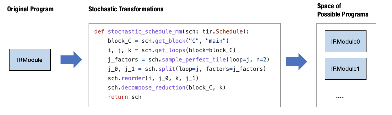
Coming back to our initial intuition, we want to be able to specify a
set of possible programs instead of one program.
stochastic_schedule_mm did exactly that. Of course, one natural
question to ask next is what is the best choice.
We will need a search algorithm to do that. To show what can be done
here, let us first try the most straightforward search algorithm –
random search, in the following code block. It tries to run
stochastic_schedule_mm repetitively, gets a transformed module, runs
benchmark, then book keep the best one in history.
def random_search(mod: tvm.IRModule, num_trials=5):
    best_result = None
    best_sch = None

    for i in range(num_trials):
        sch = stochastic_schedule_mm(tvm.tir.Schedule(mod))
        lib = tvm.build(sch.mod, target="llvm")
        f_timer_after = lib.time_evaluator("main", tvm.cpu())
        result = f_timer_after(a_nd, b_nd, c_nd).mean

        print("=====Attempt %d, time-cost: %.3f ms====" % (i, result * 1000))
        print(sch.trace)

        # book keep the best result so far
        if best_result is None or result < best_result:
            best_result = result
            best_sch = sch

    return best_sch

sch = random_search(MyModule)
=====Attempt 0, time-cost: 0.165 ms====
# from tvm import tir
def apply_trace(sch: tir.Schedule) -> None:
  b0 = sch.get_block(name="C", func_name="main")
  l1, l2, l3 = sch.get_loops(block=b0)
  v4, v5 = sch.sample_perfect_tile(loop=l2, n=2, max_innermost_factor=16, decision=[8, 16])
  l6, l7 = sch.split(loop=l2, factors=[v4, v5], preserve_unit_iters=True, disable_predication=False)
  sch.reorder(l1, l6, l3, l7)
  b8 = sch.decompose_reduction(block=b0, loop=l3)
=====Attempt 1, time-cost: 0.176 ms====
# from tvm import tir
def apply_trace(sch: tir.Schedule) -> None:
  b0 = sch.get_block(name="C", func_name="main")
  l1, l2, l3 = sch.get_loops(block=b0)
  v4, v5 = sch.sample_perfect_tile(loop=l2, n=2, max_innermost_factor=16, decision=[8, 16])
  l6, l7 = sch.split(loop=l2, factors=[v4, v5], preserve_unit_iters=True, disable_predication=False)
  sch.reorder(l1, l6, l3, l7)
  b8 = sch.decompose_reduction(block=b0, loop=l3)
=====Attempt 2, time-cost: 0.395 ms====
# from tvm import tir
def apply_trace(sch: tir.Schedule) -> None:
  b0 = sch.get_block(name="C", func_name="main")
  l1, l2, l3 = sch.get_loops(block=b0)
  v4, v5 = sch.sample_perfect_tile(loop=l2, n=2, max_innermost_factor=16, decision=[16, 8])
  l6, l7 = sch.split(loop=l2, factors=[v4, v5], preserve_unit_iters=True, disable_predication=False)
  sch.reorder(l1, l6, l3, l7)
  b8 = sch.decompose_reduction(block=b0, loop=l3)
=====Attempt 3, time-cost: 0.713 ms====
# from tvm import tir
def apply_trace(sch: tir.Schedule) -> None:
  b0 = sch.get_block(name="C", func_name="main")
  l1, l2, l3 = sch.get_loops(block=b0)
  v4, v5 = sch.sample_perfect_tile(loop=l2, n=2, max_innermost_factor=16, decision=[32, 4])
  l6, l7 = sch.split(loop=l2, factors=[v4, v5], preserve_unit_iters=True, disable_predication=False)
  sch.reorder(l1, l6, l3, l7)
  b8 = sch.decompose_reduction(block=b0, loop=l3)
=====Attempt 4, time-cost: 1.515 ms====
# from tvm import tir
def apply_trace(sch: tir.Schedule) -> None:
  b0 = sch.get_block(name="C", func_name="main")
  l1, l2, l3 = sch.get_loops(block=b0)
  v4, v5 = sch.sample_perfect_tile(loop=l2, n=2, max_innermost_factor=16, decision=[64, 2])
  l6, l7 = sch.split(loop=l2, factors=[v4, v5], preserve_unit_iters=True, disable_predication=False)
  sch.reorder(l1, l6, l3, l7)
  b8 = sch.decompose_reduction(block=b0, loop=l3)
If we run the code, we can find that it goes over a few choices and then returns the best run throughout five trials.
print(sch.trace)
# from tvm import tir
def apply_trace(sch: tir.Schedule) -> None:
  b0 = sch.get_block(name="C", func_name="main")
  l1, l2, l3 = sch.get_loops(block=b0)
  v4, v5 = sch.sample_perfect_tile(loop=l2, n=2, max_innermost_factor=16, decision=[8, 16])
  l6, l7 = sch.split(loop=l2, factors=[v4, v5], preserve_unit_iters=True, disable_predication=False)
  sch.reorder(l1, l6, l3, l7)
  b8 = sch.decompose_reduction(block=b0, loop=l3)
In practice, we use smarter algorithms. We also need to provide additional utilities, such as benchmarking on remote devices, if we are interested in optimization for other devices. TVM’s meta schedule API provides these additional capabilities.
meta_schedule is the namespace that comes to support search over a
space of possible transformations. There are many additional things that
meta-schedule do behind the scene:
Parallel benchmarking across many processes.
Use cost models to avoid benchmarking each time.
Evolutionary search on the traces instead of randomly sampling at each time.
Despite these magics, the key idea remains the same: use stochastic transformation to specify a search space of good programs, ``tune_tir`` API helps to search and find an optimized solution within the search space.
from tvm import meta_schedule as ms

database = ms.tune_tir(
    mod=MyModule,
    target="llvm --num-cores=1",
    max_trials_global=64,
    num_trials_per_iter=64,
    space=ms.space_generator.ScheduleFn(stochastic_schedule_mm),
    work_dir="./tune_tmp",
)

sch = ms.tir_integration.compile_tir(database, MyModule, "llvm --num-cores=1")
2024-10-16 14:31:55 [INFO] Logging directory: ./tune_tmp/logs
2024-10-16 14:32:04 [INFO] LocalBuilder: max_workers = 2
2024-10-16 14:32:05 [INFO] LocalRunner: max_workers = 1
2024-10-16 14:32:06 [INFO] [task_scheduler.cc:159] Initializing Task #0: "main"
| Name | FLOP | Weight | Speed (GFLOPS) | Latency (us) | Weighted Latency (us) | Trials | Done | |
|---|---|---|---|---|---|---|---|---|
| 0 | main | 4194304 | 1 | N/A | N/A | N/A | 0 |
Total trials: 0
Total latency (us): 0

2024-10-16 14:32:06 [DEBUG] [task_scheduler.cc:318]
 ID | Name |    FLOP | Weight | Speed (GFLOPS) | Latency (us) | Weighted Latency (us) | Trials | Done
------------------------------------------------------------------------------------------------------
  0 | main | 4194304 |      1 |            N/A |          N/A |                   N/A |      0 |
------------------------------------------------------------------------------------------------------
Total trials: 0
Total latency (us): 0

2024-10-16 14:32:06 [INFO] [task_scheduler.cc:180] TaskScheduler picks Task #0: "main"
2024-10-16 14:32:07 [INFO] [task_scheduler.cc:193] Sending 5 sample(s) to builder
2024-10-16 14:32:08 [INFO] [task_scheduler.cc:195] Sending 5 sample(s) to runner
2024-10-16 14:32:09 [DEBUG] XGB iter   0: tr-p-rmse: 0.327088       tr-a-peak@32: 0.931043  tr-rmse: 0.340102       tr-rmse: 0.340102
2024-10-16 14:32:09 [DEBUG] XGB iter  25: tr-p-rmse: 0.151834       tr-a-peak@32: 1.000000  tr-rmse: 0.076069       tr-rmse: 0.076069
2024-10-16 14:32:09 [DEBUG] XGB iter  50: tr-p-rmse: 0.146575       tr-a-peak@32: 1.000000  tr-rmse: 0.074000       tr-rmse: 0.074000
2024-10-16 14:32:10 [DEBUG] XGB iter  75: tr-p-rmse: 0.146401       tr-a-peak@32: 1.000000  tr-rmse: 0.074000       tr-rmse: 0.074000
2024-10-16 14:32:10 [DEBUG] XGB iter 100: tr-p-rmse: 0.146396       tr-a-peak@32: 1.000000  tr-rmse: 0.074000       tr-rmse: 0.074000
2024-10-16 14:32:10 [DEBUG] XGB iter 125: tr-p-rmse: 0.146396       tr-a-peak@32: 1.000000  tr-rmse: 0.074000       tr-rmse: 0.074000
2024-10-16 14:32:10 [DEBUG] XGB stopped. Best iteration: [98] tr-p-rmse:0.14640     tr-a-peak@32:1.00000    tr-rmse:0.07400 tr-rmse:0.07400
2024-10-16 14:32:10 [INFO] [task_scheduler.cc:237] [Updated] Task #0: "main"
| Name | FLOP | Weight | Speed (GFLOPS) | Latency (us) | Weighted Latency (us) | Trials | Done | |
|---|---|---|---|---|---|---|---|---|
| 0 | main | 4194304 | 1 | 16.8929 | 248.2878 | 248.2878 | 5 |
Total trials: 5
Total latency (us): 248.288

2024-10-16 14:32:10 [DEBUG] [task_scheduler.cc:318]
 ID | Name |    FLOP | Weight | Speed (GFLOPS) | Latency (us) | Weighted Latency (us) | Trials | Done
------------------------------------------------------------------------------------------------------
  0 | main | 4194304 |      1 |        16.8929 |     248.2878 |              248.2878 |      5 |
------------------------------------------------------------------------------------------------------
Total trials: 5
Total latency (us): 248.288

2024-10-16 14:32:10 [INFO] [task_scheduler.cc:180] TaskScheduler picks Task #0: "main"
2024-10-16 14:32:11 [INFO] [task_scheduler.cc:193] Sending 0 sample(s) to builder
2024-10-16 14:32:11 [INFO] [task_scheduler.cc:195] Sending 0 sample(s) to runner
2024-10-16 14:32:11 [INFO] [task_scheduler.cc:237] [Updated] Task #0: "main"
| Name | FLOP | Weight | Speed (GFLOPS) | Latency (us) | Weighted Latency (us) | Trials | Done | |
|---|---|---|---|---|---|---|---|---|
| 0 | main | 4194304 | 1 | 16.8929 | 248.2878 | 248.2878 | 5 |
Total trials: 5
Total latency (us): 248.288

2024-10-16 14:32:11 [DEBUG] [task_scheduler.cc:318]
 ID | Name |    FLOP | Weight | Speed (GFLOPS) | Latency (us) | Weighted Latency (us) | Trials | Done
------------------------------------------------------------------------------------------------------
  0 | main | 4194304 |      1 |        16.8929 |     248.2878 |              248.2878 |      5 |
------------------------------------------------------------------------------------------------------
Total trials: 5
Total latency (us): 248.288

2024-10-16 14:32:11 [INFO] [task_scheduler.cc:180] TaskScheduler picks Task #0: "main"
2024-10-16 14:32:12 [INFO] [task_scheduler.cc:193] Sending 0 sample(s) to builder
2024-10-16 14:32:12 [INFO] [task_scheduler.cc:195] Sending 0 sample(s) to runner
2024-10-16 14:32:12 [INFO] [task_scheduler.cc:237] [Updated] Task #0: "main"
| Name | FLOP | Weight | Speed (GFLOPS) | Latency (us) | Weighted Latency (us) | Trials | Done | |
|---|---|---|---|---|---|---|---|---|
| 0 | main | 4194304 | 1 | 16.8929 | 248.2878 | 248.2878 | 5 |
Total trials: 5
Total latency (us): 248.288

2024-10-16 14:32:12 [DEBUG] [task_scheduler.cc:318]
 ID | Name |    FLOP | Weight | Speed (GFLOPS) | Latency (us) | Weighted Latency (us) | Trials | Done
------------------------------------------------------------------------------------------------------
  0 | main | 4194304 |      1 |        16.8929 |     248.2878 |              248.2878 |      5 |
------------------------------------------------------------------------------------------------------
Total trials: 5
Total latency (us): 248.288

2024-10-16 14:32:12 [INFO] [task_scheduler.cc:180] TaskScheduler picks Task #0: "main"
2024-10-16 14:32:13 [INFO] [task_scheduler.cc:193] Sending 0 sample(s) to builder
2024-10-16 14:32:13 [INFO] [task_scheduler.cc:195] Sending 0 sample(s) to runner
2024-10-16 14:32:13 [INFO] [task_scheduler.cc:237] [Updated] Task #0: "main"
| Name | FLOP | Weight | Speed (GFLOPS) | Latency (us) | Weighted Latency (us) | Trials | Done | |
|---|---|---|---|---|---|---|---|---|
| 0 | main | 4194304 | 1 | 16.8929 | 248.2878 | 248.2878 | 5 |
Total trials: 5
Total latency (us): 248.288

2024-10-16 14:32:13 [DEBUG] [task_scheduler.cc:318]
 ID | Name |    FLOP | Weight | Speed (GFLOPS) | Latency (us) | Weighted Latency (us) | Trials | Done
------------------------------------------------------------------------------------------------------
  0 | main | 4194304 |      1 |        16.8929 |     248.2878 |              248.2878 |      5 |
------------------------------------------------------------------------------------------------------
Total trials: 5
Total latency (us): 248.288

2024-10-16 14:32:13 [INFO] [task_scheduler.cc:180] TaskScheduler picks Task #0: "main"
2024-10-16 14:32:13 [INFO] [task_scheduler.cc:193] Sending 0 sample(s) to builder
2024-10-16 14:32:13 [INFO] [task_scheduler.cc:195] Sending 0 sample(s) to runner
2024-10-16 14:32:13 [INFO] [task_scheduler.cc:237] [Updated] Task #0: "main"
| Name | FLOP | Weight | Speed (GFLOPS) | Latency (us) | Weighted Latency (us) | Trials | Done | |
|---|---|---|---|---|---|---|---|---|
| 0 | main | 4194304 | 1 | 16.8929 | 248.2878 | 248.2878 | 5 |
2024-10-16 14:32:13 [DEBUG] [task_scheduler.cc:318]
 ID | Name |    FLOP | Weight | Speed (GFLOPS) | Latency (us) | Weighted Latency (us) | Trials | Done
------------------------------------------------------------------------------------------------------
  0 | main | 4194304 |      1 |        16.8929 |     248.2878 |              248.2878 |      5 |
------------------------------------------------------------------------------------------------------
Total trials: 5
Total latency (us): 248.288


Total trials: 5
Total latency (us): 248.288

2024-10-16 14:32:13 [INFO] [task_scheduler.cc:180] TaskScheduler picks Task #0: "main"
2024-10-16 14:32:14 [INFO] [task_scheduler.cc:260] Task #0 has finished. Remaining task(s): 0
| Name | FLOP | Weight | Speed (GFLOPS) | Latency (us) | Weighted Latency (us) | Trials | Done | |
|---|---|---|---|---|---|---|---|---|
| 0 | main | 4194304 | 1 | 16.8929 | 248.2878 | 248.2878 | 5 | Y |
2024-10-16 14:32:14 [DEBUG] [task_scheduler.cc:318]
 ID | Name |    FLOP | Weight | Speed (GFLOPS) | Latency (us) | Weighted Latency (us) | Trials | Done
------------------------------------------------------------------------------------------------------
  0 | main | 4194304 |      1 |        16.8929 |     248.2878 |              248.2878 |      5 |    Y
------------------------------------------------------------------------------------------------------
Total trials: 5
Total latency (us): 248.288


Total trials: 5
Total latency (us): 248.288
tune_tir functions return an optimized schedule found during the
tuning process.
sch.trace.show()
# from tvm import tir
def apply_trace(sch: tir.Schedule) -> None:
  b0 = sch.get_block(name="C", func_name="main")
  l1, l2, l3 = sch.get_loops(block=b0)
  v4, v5 = sch.sample_perfect_tile(loop=l2, n=2, max_innermost_factor=16, decision=[8, 16])
  l6, l7 = sch.split(loop=l2, factors=[v4, v5], preserve_unit_iters=True, disable_predication=False)
  sch.reorder(l1, l6, l3, l7)
  b8 = sch.decompose_reduction(block=b0, loop=l3)
  sch.enter_postproc()
IPython.display.HTML(code2html(sch.mod.script()))
# from tvm.script import ir as I
# from tvm.script import tir as T

@I.ir_module
class Module:
    @T.prim_func
    def main(A: T.Buffer((128, 128), "float32"), B: T.Buffer((128, 128), "float32"), C: T.Buffer((128, 128), "float32")):
        T.func_attr({"tir.noalias": T.bool(True)})
        # with T.block("root"):
        for i, j_0 in T.grid(128, 8):
            for j_1_init in range(16):
                with T.block("C_init"):
                    vi = T.axis.spatial(128, i)
                    vj = T.axis.spatial(128, j_0 * 16 + j_1_init)
                    T.reads()
                    T.writes(C[vi, vj])
                    C[vi, vj] = T.float32(0.0)
            for k, j_1 in T.grid(128, 16):
                with T.block("C_update"):
                    vi = T.axis.spatial(128, i)
                    vj = T.axis.spatial(128, j_0 * 16 + j_1)
                    vk = T.axis.reduce(128, k)
                    T.reads(C[vi, vj], A[vi, vk], B[vk, vj])
                    T.writes(C[vi, vj])
                    C[vi, vj] = C[vi, vj] + A[vi, vk] * B[vk, vj]
lib = tvm.build(sch.mod, target="llvm")
f_timer_after = lib.time_evaluator("main", tvm.cpu())
print("Time cost of MyModule after tuning: %.3f ms" % (f_timer_after(a_nd, b_nd, c_nd).mean * 1000))
Time cost of MyModule after tuning: 0.177 ms
4.5.1. Leverage Default AutoScheduling
In the last section, we showed how to tune a workload with stochastic
transformations that we crafted. Metaschedule comes with its own
built-in set of generic stochastic transformations that works for a
broad set of TensorIR computations. This approach is also called
auto-scheduling, as the search space is generated by the system. We can
run it by removing the line
space=ms.space_generator.ScheduleFn(stochastic_schedule_mm).
Under the hood, the meta-scheduler analyzes each block’s data access and loop patterns and proposes stochastic transformations to the program. We won’t go into these generic transformations in this chapter but want to note that they are also just stochastic transformations coupled with an analysis of the code. We can use the same mechanisms learned in the last section to enhance auto-scheduling. We will touch base on this topic in future chapters.
database = ms.tune_tir(
    mod=MyModule,
    target="llvm --num-cores=1",
    max_trials_global=64,
    num_trials_per_iter=64,
    work_dir="./tune_tmp",
)
sch = ms.tir_integration.compile_tir(database, MyModule, "llvm --num-cores=1")
2024-10-16 14:32:14 [INFO] Logging directory: ./tune_tmp/logs
2024-10-16 14:32:14 [INFO] LocalBuilder: max_workers = 2
2024-10-16 14:32:15 [INFO] LocalRunner: max_workers = 1
2024-10-16 14:32:16 [INFO] [task_scheduler.cc:159] Initializing Task #0: "main"
| Name | FLOP | Weight | Speed (GFLOPS) | Latency (us) | Weighted Latency (us) | Trials | Done | |
|---|---|---|---|---|---|---|---|---|
| 0 | main | 4194304 | 1 | N/A | N/A | N/A | 0 |
2024-10-16 14:32:16 [DEBUG] [task_scheduler.cc:318]
 ID | Name |    FLOP | Weight | Speed (GFLOPS) | Latency (us) | Weighted Latency (us) | Trials | Done
------------------------------------------------------------------------------------------------------
  0 | main | 4194304 |      1 |            N/A |          N/A |                   N/A |      0 |
------------------------------------------------------------------------------------------------------
Total trials: 0
Total latency (us): 0


Total trials: 0
Total latency (us): 0

2024-10-16 14:32:16 [INFO] [task_scheduler.cc:180] TaskScheduler picks Task #0: "main"
2024-10-16 14:32:19 [INFO] [task_scheduler.cc:193] Sending 64 sample(s) to builder
2024-10-16 14:32:38 [INFO] [task_scheduler.cc:195] Sending 64 sample(s) to runner
2024-10-16 14:32:52 [DEBUG] XGB iter   0: tr-p-rmse: 0.393679       tr-a-peak@32: 1.000000  tr-rmse: 0.279481       tr-rmse: 0.279481
2024-10-16 14:32:52 [DEBUG] XGB iter  25: tr-p-rmse: 0.038281       tr-a-peak@32: 1.000000  tr-rmse: 0.300408       tr-rmse: 0.300408
2024-10-16 14:32:52 [DEBUG] XGB iter  50: tr-p-rmse: 0.038269       tr-a-peak@32: 1.000000  tr-rmse: 0.300430       tr-rmse: 0.300430
2024-10-16 14:32:52 [DEBUG] XGB iter  75: tr-p-rmse: 0.038269       tr-a-peak@32: 1.000000  tr-rmse: 0.300430       tr-rmse: 0.300430
2024-10-16 14:32:52 [DEBUG] XGB stopped. Best iteration: [34] tr-p-rmse:0.03827     tr-a-peak@32:1.00000    tr-rmse:0.30043 tr-rmse:0.30043
2024-10-16 14:32:53 [INFO] [task_scheduler.cc:237] [Updated] Task #0: "main"
| Name | FLOP | Weight | Speed (GFLOPS) | Latency (us) | Weighted Latency (us) | Trials | Done | |
|---|---|---|---|---|---|---|---|---|
| 0 | main | 4194304 | 1 | 32.3255 | 129.7520 | 129.7520 | 64 |
2024-10-16 14:32:53 [DEBUG] [task_scheduler.cc:318]
 ID | Name |    FLOP | Weight | Speed (GFLOPS) | Latency (us) | Weighted Latency (us) | Trials | Done
------------------------------------------------------------------------------------------------------
  0 | main | 4194304 |      1 |        32.3255 |     129.7520 |              129.7520 |     64 |
------------------------------------------------------------------------------------------------------
Total trials: 64
Total latency (us): 129.752


Total trials: 64
Total latency (us): 129.752

2024-10-16 14:32:53 [INFO] [task_scheduler.cc:260] Task #0 has finished. Remaining task(s): 0
| Name | FLOP | Weight | Speed (GFLOPS) | Latency (us) | Weighted Latency (us) | Trials | Done | |
|---|---|---|---|---|---|---|---|---|
| 0 | main | 4194304 | 1 | 32.3255 | 129.7520 | 129.7520 | 64 | Y |
2024-10-16 14:32:53 [DEBUG] [task_scheduler.cc:318]
 ID | Name |    FLOP | Weight | Speed (GFLOPS) | Latency (us) | Weighted Latency (us) | Trials | Done
------------------------------------------------------------------------------------------------------
  0 | main | 4194304 |      1 |        32.3255 |     129.7520 |              129.7520 |     64 |    Y
------------------------------------------------------------------------------------------------------
Total trials: 64
Total latency (us): 129.752


Total trials: 64
Total latency (us): 129.752
lib = tvm.build(sch.mod, target="llvm")
f_timer_after = lib.time_evaluator("main", tvm.cpu())
print("Time cost of MyModule after tuning: %.3f ms" % (f_timer_after(a_nd, b_nd, c_nd).mean * 1000))
Time cost of MyModule after tuning: 0.158 ms
The result gets much faster than our original code. We can take a glimpse at the trace and the final code. For the purpose of this chapter, you do not need to understand all the transformations. At a high level, the trace involves:
More levels of loop tiling transformations.
Vectorization of intermediate computations.
Parallelization and unrolling of loops.
sch.trace.show()
# from tvm import tir
def apply_trace(sch: tir.Schedule) -> None:
  b0 = sch.get_block(name="C", func_name="main")
  b1 = sch.get_block(name="root", func_name="main")
  sch.annotate(block_or_loop=b0, ann_key="meta_schedule.tiling_structure", ann_val="SSRSRS")
  l2, l3, l4 = sch.get_loops(block=b0)
  v5, v6, v7, v8 = sch.sample_perfect_tile(loop=l2, n=4, max_innermost_factor=64, decision=[4, 2, 16, 1])
  l9, l10, l11, l12 = sch.split(loop=l2, factors=[v5, v6, v7, v8], preserve_unit_iters=True, disable_predication=False)
  v13, v14, v15, v16 = sch.sample_perfect_tile(loop=l3, n=4, max_innermost_factor=64, decision=[2, 2, 4, 8])
  l17, l18, l19, l20 = sch.split(loop=l3, factors=[v13, v14, v15, v16], preserve_unit_iters=True, disable_predication=False)
  v21, v22 = sch.sample_perfect_tile(loop=l4, n=2, max_innermost_factor=64, decision=[64, 2])
  l23, l24 = sch.split(loop=l4, factors=[v21, v22], preserve_unit_iters=True, disable_predication=False)
  sch.reorder(l9, l17, l10, l18, l23, l11, l19, l24, l12, l20)
  b25 = sch.cache_write(block=b0, write_buffer_index=0, storage_scope="global")
  sch.reverse_compute_at(block=b25, loop=l17, preserve_unit_loops=True, index=-1)
  sch.annotate(block_or_loop=b1, ann_key="meta_schedule.parallel", ann_val=16)
  sch.annotate(block_or_loop=b1, ann_key="meta_schedule.vectorize", ann_val=64)
  v26 = sch.sample_categorical(candidates=[0, 16, 64, 512], probs=[0.25, 0.25, 0.25, 0.25], decision=0)
  sch.annotate(block_or_loop=b1, ann_key="meta_schedule.unroll_explicit", ann_val=v26)
  sch.enter_postproc()
  b27 = sch.get_block(name="root", func_name="main")
  sch.unannotate(block_or_loop=b27, ann_key="meta_schedule.parallel")
  sch.unannotate(block_or_loop=b27, ann_key="meta_schedule.vectorize")
  sch.unannotate(block_or_loop=b27, ann_key="meta_schedule.unroll_explicit")
  b28, b29 = sch.get_child_blocks(b27)
  l30, l31, l32, l33, l34, l35, l36, l37, l38, l39 = sch.get_loops(block=b28)
  l40 = sch.fuse(l30, l31, preserve_unit_iters=True)
  sch.parallel(loop=l40)
  l41 = sch.fuse(l39, preserve_unit_iters=True)
  sch.vectorize(loop=l41)
  l42, l43, l44 = sch.get_loops(block=b29)
  l45 = sch.fuse(l42, preserve_unit_iters=True)
  sch.parallel(loop=l45)
  l46 = sch.fuse(l44, preserve_unit_iters=True)
  sch.vectorize(loop=l46)
  b47 = sch.get_block(name="C", func_name="main")
  l48, l49, l50, l51, l52, l53, l54, l55, l56 = sch.get_loops(block=b47)
  b57 = sch.decompose_reduction(block=b47, loop=l51)
IPython.display.HTML(code2html(sch.mod.script()))
# from tvm.script import ir as I
# from tvm.script import tir as T

@I.ir_module
class Module:
    @T.prim_func
    def main(A: T.Buffer((128, 128), "float32"), B: T.Buffer((128, 128), "float32"), C: T.Buffer((128, 128), "float32")):
        T.func_attr({"tir.noalias": T.bool(True)})
        # with T.block("root"):
        C_global = T.alloc_buffer((128, 128))
        for i_0_j_0_fused_fused in T.parallel(8):
            for i_1, j_1 in T.grid(2, 2):
                for i_2_init, j_2_init, i_3_init in T.grid(16, 4, 1):
                    for j_3_fused_init in T.vectorized(8):
                        with T.block("C_init"):
                            vi = T.axis.spatial(128, i_0_j_0_fused_fused // 2 * 32 + i_1 * 16 + i_2_init + i_3_init)
                            vj = T.axis.spatial(128, i_0_j_0_fused_fused % 2 * 64 + j_1 * 32 + j_2_init * 8 + j_3_fused_init)
                            T.reads()
                            T.writes(C_global[vi, vj])
                            T.block_attr({"meta_schedule.tiling_structure": "SSRSRS"})
                            C_global[vi, vj] = T.float32(0.0)
                for k_0, i_2, j_2, k_1, i_3 in T.grid(64, 16, 4, 2, 1):
                    for j_3_fused in T.vectorized(8):
                        with T.block("C_update"):
                            vi = T.axis.spatial(128, i_0_j_0_fused_fused // 2 * 32 + i_1 * 16 + i_2 + i_3)
                            vj = T.axis.spatial(128, i_0_j_0_fused_fused % 2 * 64 + j_1 * 32 + j_2 * 8 + j_3_fused)
                            vk = T.axis.reduce(128, k_0 * 2 + k_1)
                            T.reads(C_global[vi, vj], A[vi, vk], B[vk, vj])
                            T.writes(C_global[vi, vj])
                            T.block_attr({"meta_schedule.tiling_structure": "SSRSRS"})
                            C_global[vi, vj] = C_global[vi, vj] + A[vi, vk] * B[vk, vj]
            for ax0 in range(32):
                for ax1_fused in T.vectorized(64):
                    with T.block("C_global"):
                        v0 = T.axis.spatial(128, i_0_j_0_fused_fused // 2 * 32 + ax0)
                        v1 = T.axis.spatial(128, i_0_j_0_fused_fused % 2 * 64 + ax1_fused)
                        T.reads(C_global[v0, v1])
                        T.writes(C[v0, v1])
                        C[v0, v1] = C_global[v0, v1]
4.5.2. Section Checkpoint
Let us have a checkpoint about what we have learned so far.
Stochastic schedule allow us to express “what are the possible transformations”.
Metaschedule’s
tune_tirAPI helps to find a good solution within the space.Metaschedule comes with a default built-in set of stochastic transformations that covers a broad range of search space.
4.6. Putting Things Back to End to End Model Execution
Up until now, we have learned to automate program optimization of a single tensor primitive function. How can we put it back and improve our end-to-end model execution?
From the MLC perspective, the automated search is a modular step, and we just need to replace the original primitive function implementation with the new one provided by the tuned result.
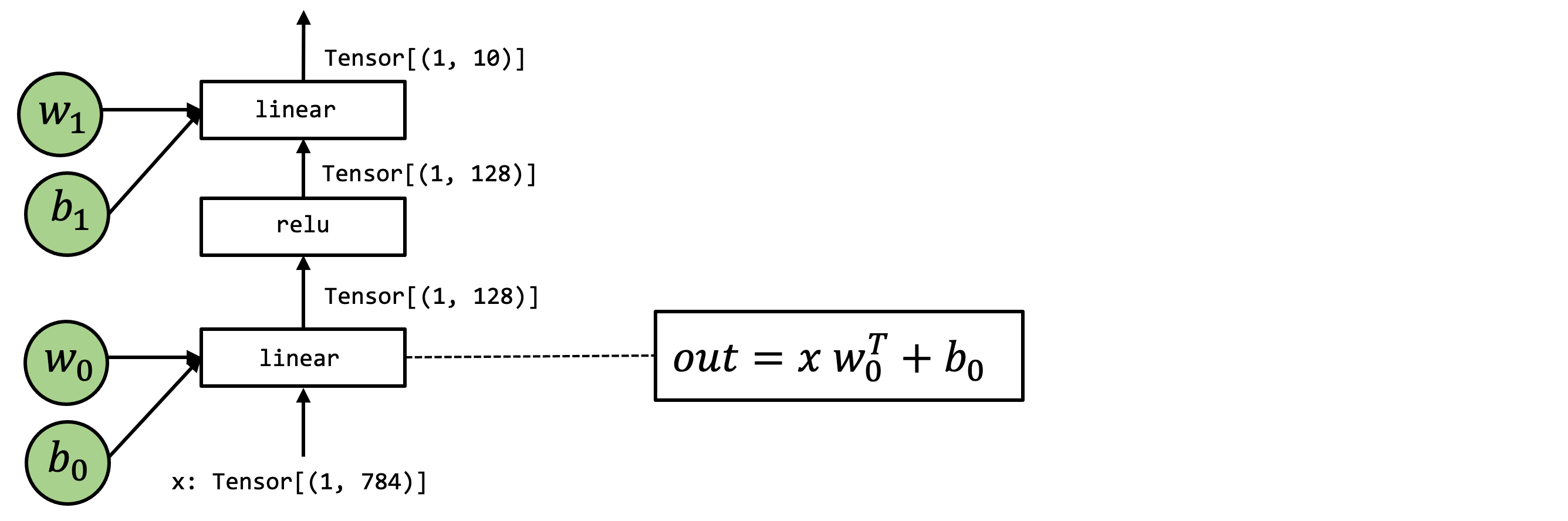
We will reuse the two-layer MLP example from the last chapter.
import torch
import torchvision

test_data = torchvision.datasets.FashionMNIST(
    root="data",
    train=False,
    download=True,
    transform=torchvision.transforms.ToTensor()
)
test_loader = torch.utils.data.DataLoader(test_data, batch_size=1, shuffle=True)
class_names = ['T-shirt/top', 'Trouser', 'Pullover', 'Dress', 'Coat',
               'Sandal', 'Shirt', 'Sneaker', 'Bag', 'Ankle boot']

img, label = next(iter(test_loader))
img = img.reshape(1, 28, 28).numpy()
Downloading http://fashion-mnist.s3-website.eu-central-1.amazonaws.com/train-images-idx3-ubyte.gz
Downloading http://fashion-mnist.s3-website.eu-central-1.amazonaws.com/train-images-idx3-ubyte.gz to data/FashionMNIST/raw/train-images-idx3-ubyte.gz
100.0%
Extracting data/FashionMNIST/raw/train-images-idx3-ubyte.gz to data/FashionMNIST/raw

Downloading http://fashion-mnist.s3-website.eu-central-1.amazonaws.com/train-labels-idx1-ubyte.gz
Downloading http://fashion-mnist.s3-website.eu-central-1.amazonaws.com/train-labels-idx1-ubyte.gz to data/FashionMNIST/raw/train-labels-idx1-ubyte.gz
100.0%
Extracting data/FashionMNIST/raw/train-labels-idx1-ubyte.gz to data/FashionMNIST/raw

Downloading http://fashion-mnist.s3-website.eu-central-1.amazonaws.com/t10k-images-idx3-ubyte.gz
Downloading http://fashion-mnist.s3-website.eu-central-1.amazonaws.com/t10k-images-idx3-ubyte.gz to data/FashionMNIST/raw/t10k-images-idx3-ubyte.gz
100.0%
Extracting data/FashionMNIST/raw/t10k-images-idx3-ubyte.gz to data/FashionMNIST/raw

Downloading http://fashion-mnist.s3-website.eu-central-1.amazonaws.com/t10k-labels-idx1-ubyte.gz
Downloading http://fashion-mnist.s3-website.eu-central-1.amazonaws.com/t10k-labels-idx1-ubyte.gz to data/FashionMNIST/raw/t10k-labels-idx1-ubyte.gz
100.0%Extracting data/FashionMNIST/raw/t10k-labels-idx1-ubyte.gz to data/FashionMNIST/raw
import matplotlib.pyplot as plt

plt.figure()
plt.imshow(img[0])
plt.colorbar()
plt.grid(False)
plt.show()

print("Class:", class_names[label[0]])
Class: Ankle boot
We also download pre-packed model parameters that we will use in our examples.
# Hide outputs
!wget -nc https://github.com/mlc-ai/web-data/raw/main/models/fasionmnist_mlp_params.pkl
As a reminder, the above figure shows the model of interest.
import pickle as pkl

mlp_params = pkl.load(open("fasionmnist_mlp_params.pkl", "rb"))

data_nd = tvm.nd.array(img.reshape(1, 784))
nd_params = {k: tvm.nd.array(v) for k, v in mlp_params.items()}
Let us use a mixture module where most of the components call into
environment function and also come with one TensorIR function
linear0.
@tvm.script.ir_module
class MyModuleMixture:
    @T.prim_func
    def linear0(X: T.Buffer((1, 784), "float32"),
                W: T.Buffer((128, 784), "float32"),
                B: T.Buffer((128,), "float32"),
                Z: T.Buffer((1, 128), "float32")):
        T.func_attr({"global_symbol": "linear0", "tir.noalias": True})
        Y = T.alloc_buffer((1, 128), "float32")
        for i, j, k in T.grid(1, 128, 784):
            with T.block("Y"):
                vi, vj, vk = T.axis.remap("SSR", [i, j, k])
                with T.init():
                    Y[vi, vj] = T.float32(0)
                Y[vi, vj] = Y[vi, vj] + X[vi, vk] * W[vj, vk]

        for i, j in T.grid(1, 128):
            with T.block("Z"):
                vi, vj = T.axis.remap("SS", [i, j])
                Z[vi, vj] =  Y[vi, vj] + B[vj]

    @R.function
    def main(x: R.Tensor((1, 784), "float32"),
             w0: R.Tensor((128, 784), "float32"),
             b0: R.Tensor((128,), "float32"),
             w1: R.Tensor((10, 128), "float32"),
             b1: R.Tensor((10,), "float32")):
        with R.dataflow():
            lv0 = R.call_dps_packed("linear0", (x, w0, b0), R.Tensor((1, 128), dtype="float32"))
            lv1 = R.call_dps_packed("env.relu", (lv0,), R.Tensor((1, 128), dtype="float32"))
            out = R.call_dps_packed("env.linear", (lv1, w1, b1), R.Tensor((1, 10), dtype="float32"))
            R.output(out)
        return out
@tvm.register_func("env.linear", override=True)
def torch_linear(x: tvm.nd.NDArray,
                 w: tvm.nd.NDArray,
                 b: tvm.nd.NDArray,
                 out: tvm.nd.NDArray):
    x_torch = torch.from_dlpack(x)
    w_torch = torch.from_dlpack(w)
    b_torch = torch.from_dlpack(b)
    out_torch = torch.from_dlpack(out)
    torch.mm(x_torch, w_torch.T, out=out_torch)
    torch.add(out_torch, b_torch, out=out_torch)

@tvm.register_func("env.relu", override=True)
def lnumpy_relu(x: tvm.nd.NDArray,
                out: tvm.nd.NDArray):
    x_torch = torch.from_dlpack(x)
    out_torch = torch.from_dlpack(out)
    torch.maximum(x_torch, torch.Tensor([0.0]), out=out_torch)
We can bind the parameters and see if it gives the correct prediction.
MyModuleWithParams = relax.transform.BindParams("main", nd_params)(MyModuleMixture)
ex = relax.build(MyModuleWithParams, target="llvm")
vm = relax.VirtualMachine(ex, tvm.cpu())

nd_res = vm["main"](data_nd)

pred_kind = np.argmax(nd_res.numpy(), axis=1)
print("MyModuleWithParams Prediction:", class_names[pred_kind[0]])
MyModuleWithParams Prediction: Ankle boot
The following code evaluates the run time cost of the module before the transformation. Note that because this is a small model, the number can fluctuate a bit between runs, so we just need to read the overall magnitude.
ftimer = vm.module.time_evaluator("main", tvm.cpu(), number=100)

print("MyModuleWithParams time-cost: %g ms" % (ftimer(data_nd).mean * 1000))
MyModuleWithParams time-cost: 0.138537 ms
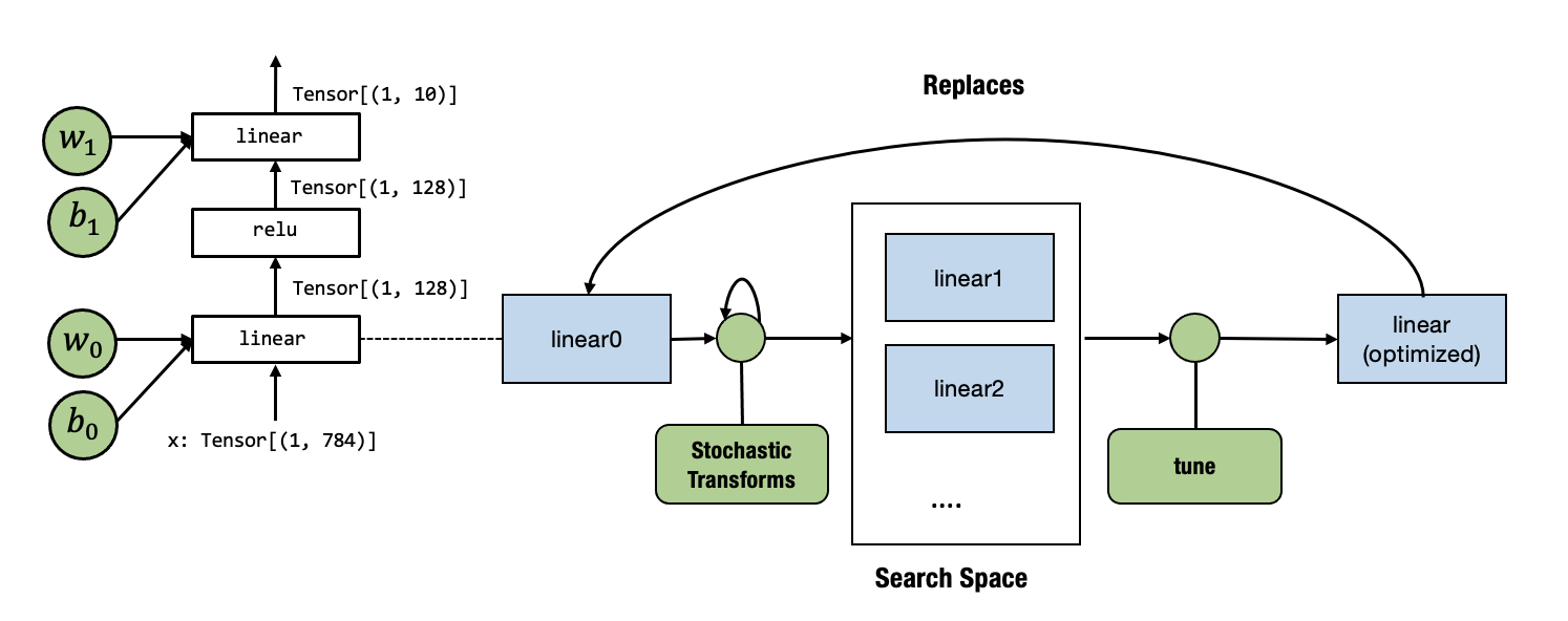
We are now ready to tune the linear0. Our overall process is
summarized in the following diagram.
Currently, tune API only takes an IRModule with one main function,
so we first get the linear0 out into another module’s main function
and pass it to tune
mod_linear = tvm.IRModule.from_expr(MyModuleMixture["linear0"].with_attr("global_symbol", "main"))
IPython.display.HTML(code2html(mod_linear.script()))
# from tvm.script import ir as I
# from tvm.script import tir as T

@I.ir_module
class Module:
    @T.prim_func
    def main(X: T.Buffer((1, 784), "float32"), W: T.Buffer((128, 784), "float32"), B: T.Buffer((128,), "float32"), Z: T.Buffer((1, 128), "float32")):
        T.func_attr({"tir.noalias": T.bool(True)})
        # with T.block("root"):
        Y = T.alloc_buffer((1, 128))
        for i, j, k in T.grid(1, 128, 784):
            with T.block("Y"):
                vi, vj, vk = T.axis.remap("SSR", [i, j, k])
                T.reads(X[vi, vk], W[vj, vk])
                T.writes(Y[vi, vj])
                with T.init():
                    Y[vi, vj] = T.float32(0.0)
                Y[vi, vj] = Y[vi, vj] + X[vi, vk] * W[vj, vk]
        for i, j in T.grid(1, 128):
            with T.block("Z"):
                vi, vj = T.axis.remap("SS", [i, j])
                T.reads(Y[vi, vj], B[vj])
                T.writes(Z[vi, vj])
                Z[vi, vj] = Y[vi, vj] + B[vj]
database = ms.tune_tir(
    mod=mod_linear,
    target="llvm --num-cores=1",
    max_trials_global=64,
    num_trials_per_iter=64,
    work_dir="./tune_tmp",
)
sch = ms.tir_integration.compile_tir(database, mod_linear, "llvm --num-cores=1")
2024-10-16 14:33:13 [INFO] Logging directory: ./tune_tmp/logs
2024-10-16 14:33:13 [INFO] LocalBuilder: max_workers = 2
2024-10-16 14:33:14 [INFO] LocalRunner: max_workers = 1
2024-10-16 14:33:15 [INFO] [task_scheduler.cc:159] Initializing Task #0: "main"
| Name | FLOP | Weight | Speed (GFLOPS) | Latency (us) | Weighted Latency (us) | Trials | Done | |
|---|---|---|---|---|---|---|---|---|
| 0 | main | 200832 | 1 | N/A | N/A | N/A | 0 |
2024-10-16 14:33:15 [DEBUG] [task_scheduler.cc:318]
 ID | Name |   FLOP | Weight | Speed (GFLOPS) | Latency (us) | Weighted Latency (us) | Trials | Done
-----------------------------------------------------------------------------------------------------
  0 | main | 200832 |      1 |            N/A |          N/A |                   N/A |      0 |
-----------------------------------------------------------------------------------------------------
Total trials: 0
Total latency (us): 0


Total trials: 0
Total latency (us): 0

2024-10-16 14:33:15 [INFO] [task_scheduler.cc:180] TaskScheduler picks Task #0: "main"
2024-10-16 14:33:18 [INFO] [task_scheduler.cc:193] Sending 64 sample(s) to builder
2024-10-16 14:33:33 [INFO] [task_scheduler.cc:195] Sending 64 sample(s) to runner
2024-10-16 14:33:50 [DEBUG] XGB iter   0: tr-p-rmse: 0.323621       tr-a-peak@32: 0.999727  tr-rmse: 0.230641       tr-rmse: 0.230641
2024-10-16 14:33:50 [DEBUG] XGB iter  25: tr-p-rmse: 0.031305       tr-a-peak@32: 1.000000  tr-rmse: 0.314151       tr-rmse: 0.314151
2024-10-16 14:33:50 [DEBUG] XGB iter  50: tr-p-rmse: 0.031299       tr-a-peak@32: 1.000000  tr-rmse: 0.314168       tr-rmse: 0.314168
2024-10-16 14:33:50 [DEBUG] XGB iter  75: tr-p-rmse: 0.031299       tr-a-peak@32: 1.000000  tr-rmse: 0.314168       tr-rmse: 0.314168
2024-10-16 14:33:51 [DEBUG] XGB stopped. Best iteration: [30] tr-p-rmse:0.03130     tr-a-peak@32:1.00000    tr-rmse:0.31417 tr-rmse:0.31417
2024-10-16 14:33:51 [INFO] [task_scheduler.cc:237] [Updated] Task #0: "main"
| Name | FLOP | Weight | Speed (GFLOPS) | Latency (us) | Weighted Latency (us) | Trials | Done | |
|---|---|---|---|---|---|---|---|---|
| 0 | main | 200832 | 1 | 8.5321 | 23.5383 | 23.5383 | 64 |
Total trials: 64
Total latency (us): 23.5383

2024-10-16 14:33:51 [DEBUG] [task_scheduler.cc:318]
 ID | Name |   FLOP | Weight | Speed (GFLOPS) | Latency (us) | Weighted Latency (us) | Trials | Done
-----------------------------------------------------------------------------------------------------
  0 | main | 200832 |      1 |         8.5321 |      23.5383 |               23.5383 |     64 |
-----------------------------------------------------------------------------------------------------
Total trials: 64
Total latency (us): 23.5383

2024-10-16 14:33:51 [INFO] [task_scheduler.cc:260] Task #0 has finished. Remaining task(s): 0
| Name | FLOP | Weight | Speed (GFLOPS) | Latency (us) | Weighted Latency (us) | Trials | Done | |
|---|---|---|---|---|---|---|---|---|
| 0 | main | 200832 | 1 | 8.5321 | 23.5383 | 23.5383 | 64 | Y |
2024-10-16 14:33:51 [DEBUG] [task_scheduler.cc:318]
 ID | Name |   FLOP | Weight | Speed (GFLOPS) | Latency (us) | Weighted Latency (us) | Trials | Done
-----------------------------------------------------------------------------------------------------
  0 | main | 200832 |      1 |         8.5321 |      23.5383 |               23.5383 |     64 |    Y
-----------------------------------------------------------------------------------------------------
Total trials: 64
Total latency (us): 23.5383


Total trials: 64
Total latency (us): 23.5383
Now we need to replace the original linear0 with the new function
after tuning. We can do that by first getting a global_var, a
pointer reference to the functions inside the IRModule, then calling
update_func to replace the function with the new one.
MyModuleWithParams2 = relax.transform.BindParams("main", nd_params)(MyModuleMixture)
new_func = sch.mod["main"].with_attr("global_symbol", "linear0")
gv = MyModuleWithParams2.get_global_var("linear0")
MyModuleWithParams2.update_func(gv, new_func)
IPython.display.HTML(code2html(MyModuleWithParams2.script()))
# from tvm.script import ir as I
# from tvm.script import tir as T
# from tvm.script import relax as R

@I.ir_module
class Module:
    @T.prim_func
    def linear0(X: T.Buffer((1, 784), "float32"), W: T.Buffer((128, 784), "float32"), B: T.Buffer((128,), "float32"), Z: T.Buffer((1, 128), "float32")):
        T.func_attr({"tir.noalias": T.bool(True)})
        # with T.block("root"):
        Y = T.alloc_buffer((1, 128))
        for i_0 in T.serial(1, annotations={"pragma_auto_unroll_max_step": 64, "pragma_unroll_explicit": 1}):
            for j_0 in range(1):
                for i_1, j_1 in T.grid(1, 8):
                    for i_2_init, j_2_init, i_3_init in T.grid(1, 1, 1):
                        for j_3_fused_init in T.vectorized(16):
                            with T.block("Y_init"):
                                vi = T.axis.spatial(1, i_0 + i_1 + i_2_init + i_3_init)
                                vj = T.axis.spatial(128, j_0 * 128 + j_1 * 16 + j_2_init * 16 + j_3_fused_init)
                                T.reads()
                                T.writes(Y[vi, vj])
                                T.block_attr({"meta_schedule.tiling_structure": "SSRSRS"})
                                Y[vi, vj] = T.float32(0.0)
                    for k_0, i_2, j_2, k_1, i_3 in T.grid(112, 1, 1, 7, 1):
                        for j_3_fused in T.vectorized(16):
                            with T.block("Y_update"):
                                vi = T.axis.spatial(1, i_0 + i_1 + i_2 + i_3)
                                vj = T.axis.spatial(128, j_0 * 128 + j_1 * 16 + j_2 * 16 + j_3_fused)
                                vk = T.axis.reduce(784, k_0 * 7 + k_1)
                                T.reads(Y[vi, vj], X[vi, vk], W[vj, vk])
                                T.writes(Y[vi, vj])
                                T.block_attr({"meta_schedule.tiling_structure": "SSRSRS"})
                                Y[vi, vj] = Y[vi, vj] + X[vi, vk] * W[vj, vk]
                for ax0, ax1 in T.grid(1, 128):
                    with T.block("Z"):
                        vi, vj = T.axis.remap("SS", [ax0, ax1])
                        T.reads(Y[vi, vj], B[vj])
                        T.writes(Z[vi, vj])
                        Z[vi, vj] = Y[vi, vj] + B[vj]

    @R.function
    def main(x: R.Tensor((1, 784), dtype="float32")) -> R.Tensor((1, 10), dtype="float32"):
        with R.dataflow():
            lv0 = R.call_dps_packed("linear0", (x, metadata["relax.expr.Constant"][0], metadata["relax.expr.Constant"][1]), out_sinfo=R.Tensor((1, 128), dtype="float32"))
            lv1 = R.call_dps_packed("env.relu", (lv0,), out_sinfo=R.Tensor((1, 128), dtype="float32"))
            out = R.call_dps_packed("env.linear", (lv1, metadata["relax.expr.Constant"][2], metadata["relax.expr.Constant"][3]), out_sinfo=R.Tensor((1, 10), dtype="float32"))
            R.output(out)
        return out

# Metadata omitted. Use show_meta=True in script() method to show it.
We can find that the linear0 has been replaced in the above code.
ex = relax.build(MyModuleWithParams2, target="llvm")
vm = relax.VirtualMachine(ex, tvm.cpu())

nd_res = vm["main"](data_nd)

pred_kind = np.argmax(nd_res.numpy(), axis=1)
print("MyModuleWithParams2 Prediction:", class_names[pred_kind[0]])
MyModuleWithParams2 Prediction: Ankle boot
Running the code again, we can find that we get an observable amount of
time reduction, mainly thanks to the new linear0 function.
ftimer = vm.module.time_evaluator("main", tvm.cpu(), number=50)

print("MyModuleWithParams2 time-cost: %g ms" % (ftimer(data_nd).mean * 1000))
MyModuleWithParams2 time-cost: 0.0718722 ms
4.7. Discussions
We might notice that our previous two chapters focused on abstraction while this chapter starts to focus on transformation. Stochastic transformations specify what can be possibly optimized without nailing down all the choices. The meta-schedule API helps us to search over the space of possible transformations and pick the best one.
Importantly, putting the search result back into the end-to-end flow is just a matter of replacing the implementation of the original function with a new one that is informed by the tuning process.
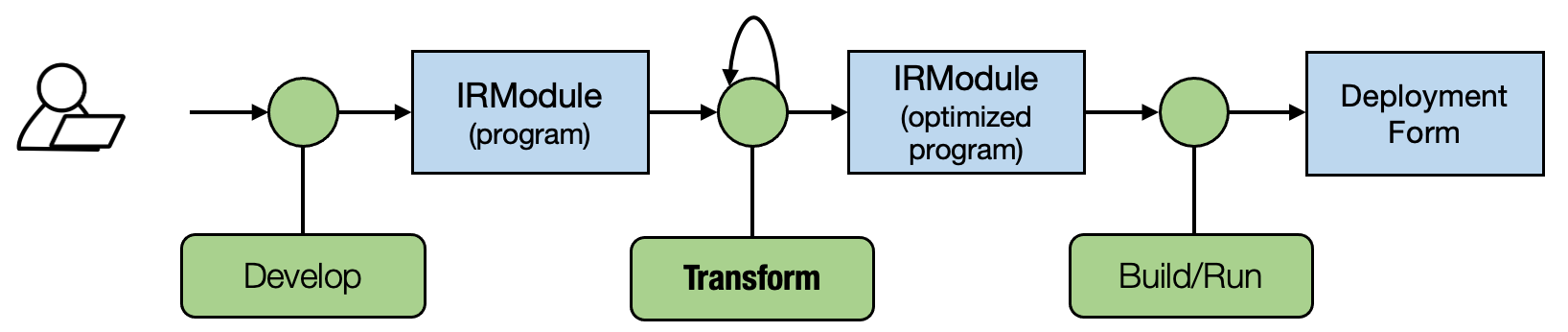
So we again are following the generic MLC process in the figure below. In future lectures, we will introduce more kinds of transformations on primitive functions and computational graph functions. A good MLC process composes these transformations together to form an end deployment form.
4.8. Summary
Stochastic transformations help us to specify a search space of possible programs.
MetaSchedule searches over the search space and finds an optimized one.
We can use another transformation to replace the primitive tensor function with optimized ones and an updated end-to-end execution flow.