2.4. TensorIR: Tensor Program Abstraction Case Study
2.4.1. Install Packages
For the purpose of this course, we will use some on-going development in tvm, which is an open source machine learning compilation framework. We provide the following command to install a packaged version for mlc course.
python3 -m pip install mlc-ai-nightly -f https://mlc.ai/wheels
2.4.2. Prelude
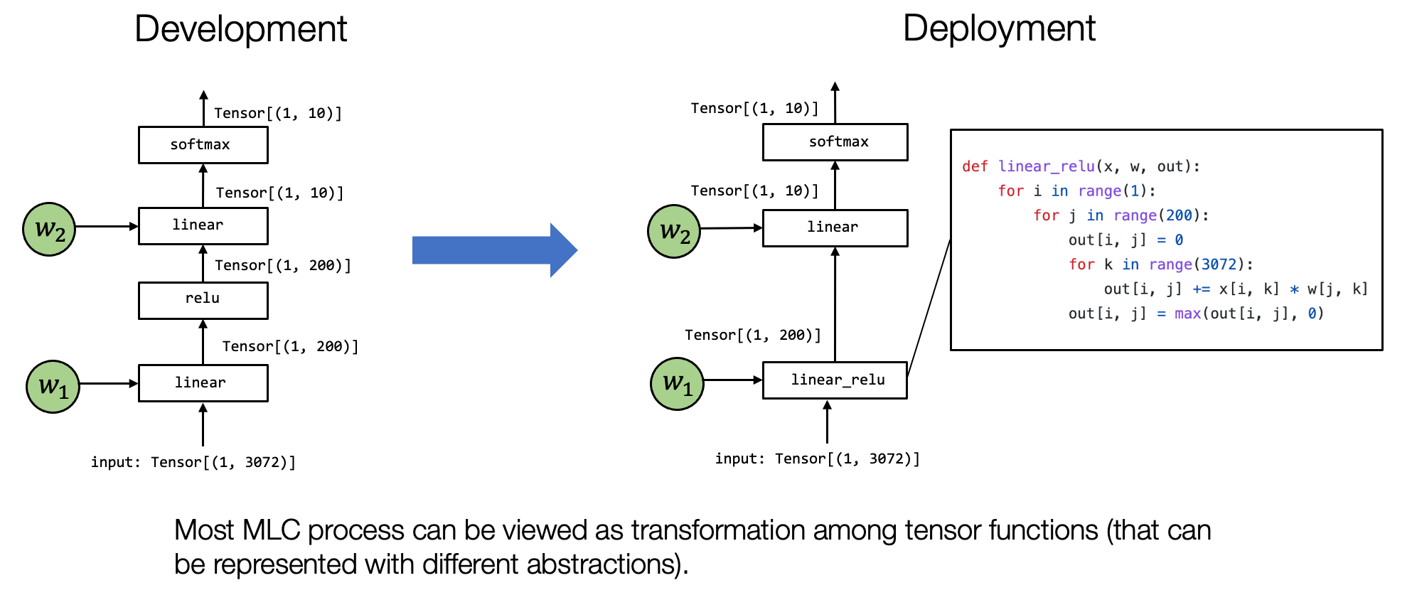
To begin today’s lecture, let us recap the key principle of the MLC process. Most of the MLC process can be viewed as transformation among tensor functions. The main thing we aim to answer in our following up are:
What are the possible abstractions to represent the tensor function.
What are possible transformations among the tensor functions.
Today we are going to cover part of that by focusing on primitive tensor functions.
2.4.3. Learning one Tensor Program Abstraction – TensorIR
We have gone over the primitive tensor function and discussed the high-level idea of tensor program abstractions.
Now we are ready to learn one specific instance of tensor program abstraction called TensorIR. TensorIR is the tensor program abstraction in Apache TVM, which is one of the standard machine learning compilation frameworks.
import numpy as np
import tvm
from tvm.ir.module import IRModule
from tvm.script import tir as T
The primary purpose of tensor program abstraction is to represent loops and corresponding hardware acceleration choices such as threading, use of specialized hardware instructions, and memory access.
To help our explanations, let us use the following sequence of tensor computations as a motivating example.
Specifically, for two \(128 \times 128\) matrices A and B, let us perform the following two steps of tensor computations.
\(Y_{i, j} = \sum_k A_{i, k} \times B_{k, j}\)
\(C_{i, j} = \mathbb{relu}(Y_{i, j}) = \mathbb{max}(Y_{i, j}, 0)\)
The above computations resemble a typical primitive tensor function commonly seen in neural networks – a linear layer with relu activation. To begin with, we can implement the two operations using array computations in NumPy as follows.
dtype = "float32"
a_np = np.random.rand(128, 128).astype(dtype)
b_np = np.random.rand(128, 128).astype(dtype)
# a @ b is equivalent to np.matmul(a, b)
c_mm_relu = np.maximum(a_np @ b_np, 0)
Under the hood, NumPy calls into libraries (such as OpenBLAS) and some of its own implementations in lower-level C languages to execute these computations.
From the tensor program abstraction point of view, we would like to see through the details under the hood of these array computations. Specifically, we want to ask: what are the possible ways to implement the corresponding computations?
For the purpose of illustrating details under the hood, we will write examples in a restricted subset of NumPy API – which we call low-level numpy that uses the following conventions:
We will use a loop instead of array functions when necessary to demonstrate the possible loop computations.
When possible, we always explicitly allocate arrays via numpy.empty and pass them around.
Note that this is not how one would typically write NumPy programs.
Still, they closely resemble what happens under the hood – most
real-world deployment solutions handle allocations separately from
computations. The specific libraries perform the computation using
different forms of loops and arithmetic computations. Of course,
primarily, they are implemented using lower-level languages such as
C.
def lnumpy_mm_relu(A: np.ndarray, B: np.ndarray, C: np.ndarray):
    Y = np.empty((128, 128), dtype="float32")
    for i in range(128):
        for j in range(128):
            for k in range(128):
                if k == 0:
                    Y[i, j] = 0
                Y[i, j] = Y[i, j] + A[i, k] * B[k, j]
    for i in range(128):
        for j in range(128):
            C[i, j] = max(Y[i, j], 0)
The program above is one way to implement the mm_relu operation. The
program contains two stages: first we allocate an intermediate storage
\(Y\) and store the result of matrix multiplication there. Then we
compute the relu in a second sequence of for loops. One thing you might
notice is that this is certainly not the only way to implement the
mm_relu. Likely this is also not the first thing that you might come
up with on top of your mind.
Nevertheless, this is one way to implement mm_relu, we can verify
the correctness of the code by comparing our result to the original one
using array computation. We will come back and revisit other possible
ways in the later part of this tutorial.
c_np = np.empty((128, 128), dtype=dtype)
lnumpy_mm_relu(a_np, b_np, c_np)
np.testing.assert_allclose(c_mm_relu, c_np, rtol=1e-5)
The above example code shows how we can bring an under the hood
implementation of mm_relu. Of course, the code itself will run much
slower because of the python interpreter. Nevertheless, the example
numpy code contains all the possible elements we will use in real-world
implementations of those computations.
Multi-dimensional buffer (arrays).
Loops over array dimensions.
Computations statements are executed under the loops.
With the low-level NumPy example in mind, now we are ready to introduce
TensorIR. The code block below shows a TensorIR implementation of
mm_relu. The particular code is implemented in a language called
TVMScript, which is a domain-specific dialect embedded in python AST.
@tvm.script.ir_module
class MyModule:
    @T.prim_func
    def mm_relu(A: T.Buffer((128, 128), "float32"),
                B: T.Buffer((128, 128), "float32"),
                C: T.Buffer((128, 128), "float32")):
        T.func_attr({"global_symbol": "mm_relu", "tir.noalias": True})
        Y = T.alloc_buffer((128, 128), dtype="float32")
        for i, j, k in T.grid(128, 128, 128):
            with T.block("Y"):
                vi = T.axis.spatial(128, i)
                vj = T.axis.spatial(128, j)
                vk = T.axis.reduce(128, k)
                with T.init():
                    Y[vi, vj] = T.float32(0)
                Y[vi, vj] = Y[vi, vj] + A[vi, vk] * B[vk, vj]
        for i, j in T.grid(128, 128):
            with T.block("C"):
                vi = T.axis.spatial(128, i)
                vj = T.axis.spatial(128, j)
                C[vi, vj] = T.max(Y[vi, vj], T.float32(0))
It is helpful to be able to see the numpy code and the TensorIR code side-by-side and check the corresponding elements, and we are going to walk through each of them in detail.
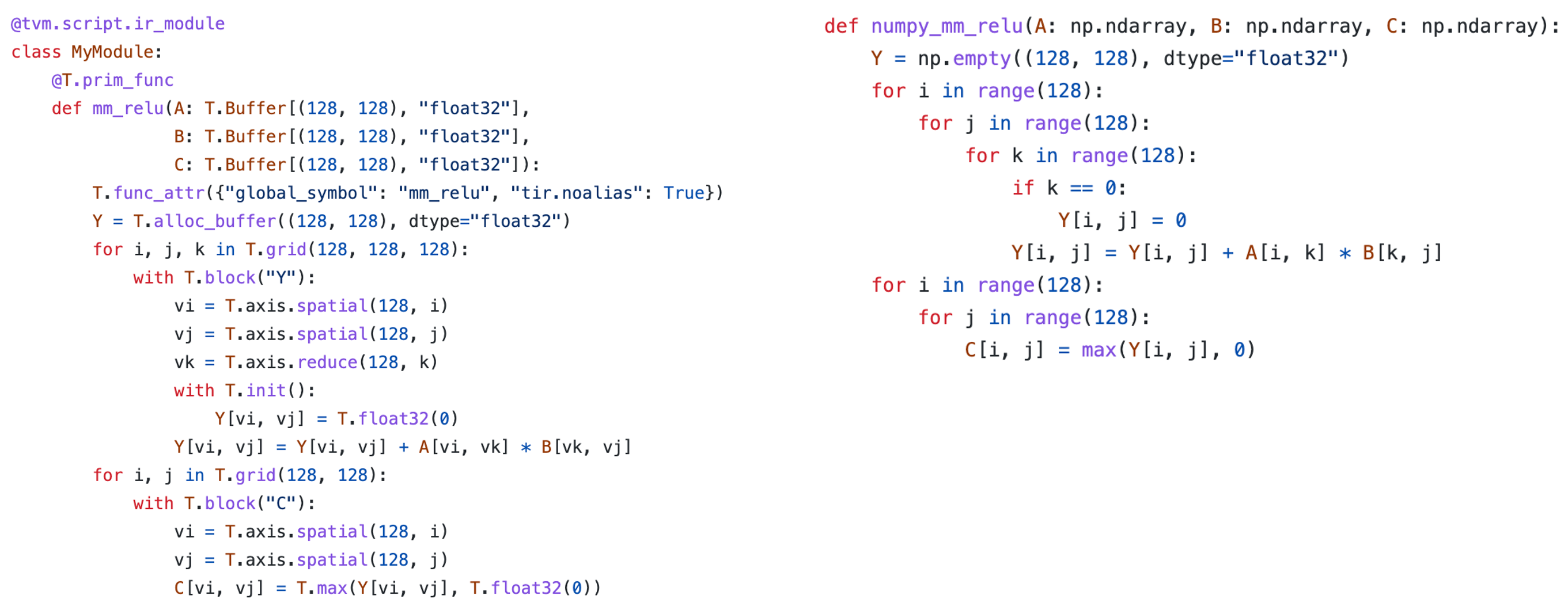
Let us first start by reviewing elements that have a direct correspondence between the numpy and TensorIR side. Then we will come back and review additional elements that are not part of the numpy program.
2.4.3.1. Function Parameters and Buffers
First, let us see the function parameters. The function parameters correspond to the same set of parameters on the numpy function.
# TensorIR
def mm_relu(A: T.Buffer[(128, 128), "float32"],
            B: T.Buffer[(128, 128), "float32"],
            C: T.Buffer[(128, 128), "float32"]):
    ...
# numpy
def lnumpy_mm_relu(A: np.ndarray, B: np.ndarray, C: np.ndarray):
    ...
Here A, B, and C takes a type named T.Buffer, which with shape
argument (128, 128) and data type float32. This additional
information helps possible MLC process to generate code that specializes
in the shape and data type.
Similarly, TensorIR also uses a buffer type in intermediate result allocation.
# TensorIR
Y = T.alloc_buffer((128, 128), dtype="float32")
# numpy
Y = np.empty((128, 128), dtype="float32")
2.4.3.2. For Loop Iterations
There are also direct correspondence of loop iterations. T.grid is a
syntactic sugar in TensorIR for us to write multiple nested iterators.
# TensorIR
for i, j, k in T.grid(128, 128, 128):

# numpy
for i in range(128):
    for j in range(128):
        for k in range(128):
2.4.3.3. Computational Block
One of the main differences comes from the computational statement.
TensorIR contains an additional construct called T.block.
# TensorIR
with T.block("Y"):
    vi = T.axis.spatial(128, i)
    vj = T.axis.spatial(128, j)
    vk = T.axis.reduce(128, k)
    with T.init():
        Y[vi, vj] = T.float32(0)
    Y[vi, vj] = Y[vi, vj] + A[vi, vk] * B[vk, vj]

# coressponding numpy code
vi, vj, vk = i, j, k
if vk == 0:
    Y[vi, vj] = 0
Y[vi, vj] = Y[vi, vj] + A[vi, vk] * B[vk, vj]
A block is a basic unit of computation in TensorIR. Notably, the
block contains a few additional pieces of information compared to the
plain NumPy code. A block contains a set of block axes (vi, vj, vk)
and computations defined around them.
vi = T.axis.spatial(128, i)
vj = T.axis.spatial(128, j)
vk = T.axis.reduce(128, k)
The above three lines declare the key properties about block axes in the following syntax.
[block_axis] = T.axis.[axis_type]([axis_range], [mapped_value])
The three lines contain the following information:
They define where should vi, vj, vk be bound to (in this case i, j k).
They declare the original range that the vi, vj, vk are supposed to be (the
128inT.axis.spatial(128, i))They declare the properties of the iterators (
spatial,reduce)
Let us walk through those property one by one. First of all, in terms of
the bounding relation. vi = T.axis.spatial(128, i) effectively
implies vi = i. The [axis_range] value provided the expected
range of the [block_axis]. For example, 128 in
vi = T.axis.spatial(128, i) provides an indication that vi
should be in the range(0, 128).
2.4.3.4. Block Axis Properties
Let us now start to take a closer look at the block axis properties.
These axis properties marks the relation of the axis to the computation
being performed. The figure below summarizes the block (iteration) axes
and the read write relations of block Y. Note that strictly speaking the
block is doing (reduction) updates to Y, we mark this as write for
now as we don’t need value of Y from another block.
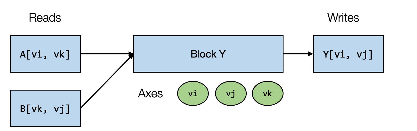
In our example, block Y computes the result Y[vi, vj] by reading
values from A[vi, vk] and B[vk, vj] and perform sum over all
possible vk. In this particular example, if we fix vi, vj to
be (0, 1), and run the block for vk in range(0, 128), we can
effectively compute C[0, 1] independently from other possible
locations (that have different values of vi, vj).
Notably, for a fixed value of vi and vj, the computation block produces
a point value at a spatial location of Y (Y[vi, vj]) that is
independent from other locations in Y (with a different vi, vj
values). We can call vi, vj spatial axes as they directly
correspond to the beginning of a spatial region of buffers that the
block writes to. The axes involved in reduction (vk) are named
reduce axes.
2.4.3.5. Why Extra Information in Block
One crucial observation is that the additional information (block axis
range and their properties) makes the block self-contained when it
comes to the iterations that it is supposed to carry out independently
from the external loop-nest i, j, k.
The block axis information also provides additional properties that help
us validate the correctness of the external loops used to carry out the
computation. For example, the code block below will result in an error
because the loop expects an iterator of size 128, but we only bound
it to a for loop of size 127.
# wrong program due to loop and block iteration mismatch
for i in range(127):
    with T.block("C"):
        vi = T.axis.spatial(128, i)
        ^^^^^^^^^^^^^^^^^^^^^^^^^^^
        error here due to iterator size mismatch
        ...
This additional information also helps us in following machine learning compilation analysis. For example, while we can always parallelize over spatial axes, parallelizing over reduce axes will require specific strategies.
2.4.3.6. Sugar for Block Axes Binding
In situations where each of the block axes is directly mapped to an
outer loop iterator, we can use T.axis.remap to declare the block
axis in a single line.
# SSR means the properties of each axes are "spatial", "spatial", "reduce"
vi, vj, vk = T.axis.remap("SSR", [i, j, k])
is equivalent to
vi = T.axis.spatial(range_of_i, i)
vj = T.axis.spatial(range_of_j, j)
vk = T.axis.reduce(range_of_k, k)
So we can also write the programs as follows.
@tvm.script.ir_module
class MyModuleWithAxisRemapSugar:
    @T.prim_func
    def mm_relu(A: T.Buffer((128, 128), "float32"),
                B: T.Buffer((128, 128), "float32"),
                C: T.Buffer((128, 128), "float32")):
        T.func_attr({"global_symbol": "mm_relu", "tir.noalias": True})
        Y = T.alloc_buffer((128, 128), dtype="float32")
        for i, j, k in T.grid(128, 128, 128):
            with T.block("Y"):
                vi, vj, vk = T.axis.remap("SSR", [i, j, k])
                with T.init():
                    Y[vi, vj] = T.float32(0)
                Y[vi, vj] = Y[vi, vj] + A[vi, vk] * B[vk, vj]
        for i, j in T.grid(128, 128):
            with T.block("C"):
                vi, vj = T.axis.remap("SS", [i, j])
                C[vi, vj] = T.max(Y[vi, vj], T.float32(0))
2.4.3.7. Function Attributes and Decorators
So far, we have covered most of the elements in TensorIR. In this part, we will go over the remaining elements of the script.
The function attribute information contains extra information about the function.
T.func_attr({"global_symbol": "mm_relu", "tir.noalias": True})
Here global_symbol corresponds to the name of the function, and
tir.noalias is an attribute indicating that all the buffer memory
areas do not overlap. You also feel free safely skip these attributes
for now as they won’t affect the overall understanding of the high-level
concepts.
The two decorators, @tvm.script.ir_module and @T.prim_func are
used to indicate the type of the corresponding part.
@tvm.script.ir_module indicates that MyModule is an IRModule.
IRModule is the container object to hold a collection of tensor
functions in machine learning compilation.
type(MyModule)
tvm.ir.module.IRModule
type(MyModule["mm_relu"])
tvm.tir.function.PrimFunc
Up until now, we have only seen IRModules containing a single tensor function. An IRModule in the MLC process can contain multiple tensor functions. The following code block shows an example of an IRModule with two functions.
@tvm.script.ir_module
class MyModuleWithTwoFunctions:
    @T.prim_func
    def mm(A: T.Buffer((128, 128), "float32"),
           B: T.Buffer((128, 128), "float32"),
           Y: T.Buffer((128, 128), "float32")):
        T.func_attr({"global_symbol": "mm", "tir.noalias": True})
        for i, j, k in T.grid(128, 128, 128):
            with T.block("Y"):
                vi, vj, vk = T.axis.remap("SSR", [i, j, k])
                with T.init():
                    Y[vi, vj] = T.float32(0)
                Y[vi, vj] = Y[vi, vj] + A[vi, vk] * B[vk, vj]

    @T.prim_func
    def relu(A: T.Buffer((128, 128), "float32"),
             B: T.Buffer((128, 128), "float32")):
        T.func_attr({"global_symbol": "relu", "tir.noalias": True})
        for i, j in T.grid(128, 128):
            with T.block("B"):
                vi, vj = T.axis.remap("SS", [i, j])
                B[vi, vj] = T.max(A[vi, vj], T.float32(0))
2.4.3.8. Section Checkpoint
So far, we have gone through one example instance of TensorIR program and covered most of the elements, including:
Buffer declarations in parameters and intermediate temporary memory.
For loop iterations.
Blocks and block axes properties.
In this section, we have gone through one example instance of TensorIR that covers the most common elements in MLC.
TensorIR contains more elements than what we went over in this section, but this section covers most of the key parts that can get us started in the MLC journey. We will cover new elements as we encounter them in the later chapters.
2.4.4. Transformation
In the last section, we learned about TensorIR and its key elements. Now, let us get to the main ingredients of all MLC flows – transformations of primitive tensor functions.
In the last section, we have given an example of how to write
mm_relu using low-level numpy. In practice, there can be multiple
ways to implement the same functionality, and each implementation can
result in different performance.
We will discuss the reason behind the performance difference and how to leverage those variants in future lectures. In this lecture, let us focus on the ability to get different implementation variants using transformations.
def lnumpy_mm_relu_v2(A: np.ndarray, B: np.ndarray, C: np.ndarray):
    Y = np.empty((128, 128), dtype="float32")
    for i in range(128):
        for j0 in range(32):
            for k in range(128):
                for j1 in range(4):
                    j = j0 * 4 + j1
                    if k == 0:
                        Y[i, j] = 0
                    Y[i, j] = Y[i, j] + A[i, k] * B[k, j]
    for i in range(128):
        for j in range(128):
            C[i, j] = max(Y[i, j], 0)

c_np = np.empty((128, 128), dtype=dtype)
lnumpy_mm_relu_v2(a_np, b_np, c_np)
np.testing.assert_allclose(c_mm_relu, c_np, rtol=1e-5)
The above code block shows a slightly different variation of
mm_relu. To see the relation to the original program
We replace the
jloop with two loops,j0andj1.The order of iterations changes slightly
In order to get lnumpy_mm_relu_v2, we have to rewrite it into a new
function (or manually copy-paste and edit). TensorIR introduces a
utility called Schedule that allows us to do that pragmatically.
To remind ourselves, let us look again at the current MyModule content.
import IPython

IPython.display.Code(MyModule.script(), language="python")
# from tvm.script import ir as I
# from tvm.script import tir as T

@I.ir_module
class Module:
    @T.prim_func
    def mm_relu(A: T.Buffer((128, 128), "float32"), B: T.Buffer((128, 128), "float32"), C: T.Buffer((128, 128), "float32")):
        T.func_attr({"tir.noalias": T.bool(True)})
        # with T.block("root"):
        Y = T.alloc_buffer((128, 128))
        for i, j, k in T.grid(128, 128, 128):
            with T.block("Y"):
                vi, vj, vk = T.axis.remap("SSR", [i, j, k])
                T.reads(A[vi, vk], B[vk, vj])
                T.writes(Y[vi, vj])
                with T.init():
                    Y[vi, vj] = T.float32(0.0)
                Y[vi, vj] = Y[vi, vj] + A[vi, vk] * B[vk, vj]
        for i, j in T.grid(128, 128):
            with T.block("C"):
                vi, vj = T.axis.remap("SS", [i, j])
                T.reads(Y[vi, vj])
                T.writes(C[vi, vj])
                C[vi, vj] = T.max(Y[vi, vj], T.float32(0.0))
Now we are ready to try out the code transformations, we begin by
creating a Schedule helper class with the given MyModule as input.
sch = tvm.tir.Schedule(MyModuleWithAxisRemapSugar)
Then we perform the following operations to obtain a reference to block Y and corresponding loops.
block_Y = sch.get_block("Y", func_name="mm_relu")
i, j, k = sch.get_loops(block_Y)
Now we are ready to perform the transformations. The first
transformation we will perform is to split the loop j into two
loops, with the length of the inner loop to be 4. Note that the
transformation is procedural, so if you accidentally execute the block
twice, we will get an error that variable j no longer exists. If
that happens, you can run again from the beginning (where sch get
created).
j0, j1 = sch.split(j, factors=[None, 4])
We can look at the result of the transformation, which is stored at
sch.mod.
IPython.display.Code(sch.mod.script(), language="python")
# from tvm.script import ir as I
# from tvm.script import tir as T

@I.ir_module
class Module:
    @T.prim_func
    def mm_relu(A: T.Buffer((128, 128), "float32"), B: T.Buffer((128, 128), "float32"), C: T.Buffer((128, 128), "float32")):
        T.func_attr({"tir.noalias": T.bool(True)})
        # with T.block("root"):
        Y = T.alloc_buffer((128, 128))
        for i, j_0, j_1, k in T.grid(128, 32, 4, 128):
            with T.block("Y"):
                vi = T.axis.spatial(128, i)
                vj = T.axis.spatial(128, j_0 * 4 + j_1)
                vk = T.axis.reduce(128, k)
                T.reads(A[vi, vk], B[vk, vj])
                T.writes(Y[vi, vj])
                with T.init():
                    Y[vi, vj] = T.float32(0.0)
                Y[vi, vj] = Y[vi, vj] + A[vi, vk] * B[vk, vj]
        for i, j in T.grid(128, 128):
            with T.block("C"):
                vi, vj = T.axis.remap("SS", [i, j])
                T.reads(Y[vi, vj])
                T.writes(C[vi, vj])
                C[vi, vj] = T.max(Y[vi, vj], T.float32(0.0))
After the first step of transformation, we created two additional loops,
j_0 and j_1, with corresponding ranges 32 and 4. Our next step
would be to reorder the two loops.
sch.reorder(j0, k, j1)
IPython.display.Code(sch.mod.script(), language="python")
# from tvm.script import ir as I
# from tvm.script import tir as T

@I.ir_module
class Module:
    @T.prim_func
    def mm_relu(A: T.Buffer((128, 128), "float32"), B: T.Buffer((128, 128), "float32"), C: T.Buffer((128, 128), "float32")):
        T.func_attr({"tir.noalias": T.bool(True)})
        # with T.block("root"):
        Y = T.alloc_buffer((128, 128))
        for i, j_0, k, j_1 in T.grid(128, 32, 128, 4):
            with T.block("Y"):
                vi = T.axis.spatial(128, i)
                vj = T.axis.spatial(128, j_0 * 4 + j_1)
                vk = T.axis.reduce(128, k)
                T.reads(A[vi, vk], B[vk, vj])
                T.writes(Y[vi, vj])
                with T.init():
                    Y[vi, vj] = T.float32(0.0)
                Y[vi, vj] = Y[vi, vj] + A[vi, vk] * B[vk, vj]
        for i, j in T.grid(128, 128):
            with T.block("C"):
                vi, vj = T.axis.remap("SS", [i, j])
                T.reads(Y[vi, vj])
                T.writes(C[vi, vj])
                C[vi, vj] = T.max(Y[vi, vj], T.float32(0.0))
Now code after reordering closely resembles lnumpy_mm_relu_v2.
2.4.4.1. Getting to Another Variant
In this section, we are going to go ahead and do another two steps of
transformations to get to another variant. First, we use a primitive
called reverse_compute_at to move block C to an inner loop of Y.
block_C = sch.get_block("C", "mm_relu")
sch.reverse_compute_at(block_C, j0)
IPython.display.Code(sch.mod.script(), language="python")
# from tvm.script import ir as I
# from tvm.script import tir as T

@I.ir_module
class Module:
    @T.prim_func
    def mm_relu(A: T.Buffer((128, 128), "float32"), B: T.Buffer((128, 128), "float32"), C: T.Buffer((128, 128), "float32")):
        T.func_attr({"tir.noalias": T.bool(True)})
        # with T.block("root"):
        Y = T.alloc_buffer((128, 128))
        for i, j_0 in T.grid(128, 32):
            for k, j_1 in T.grid(128, 4):
                with T.block("Y"):
                    vi = T.axis.spatial(128, i)
                    vj = T.axis.spatial(128, j_0 * 4 + j_1)
                    vk = T.axis.reduce(128, k)
                    T.reads(A[vi, vk], B[vk, vj])
                    T.writes(Y[vi, vj])
                    with T.init():
                        Y[vi, vj] = T.float32(0.0)
                    Y[vi, vj] = Y[vi, vj] + A[vi, vk] * B[vk, vj]
            for ax0 in range(4):
                with T.block("C"):
                    vi = T.axis.spatial(128, i)
                    vj = T.axis.spatial(128, j_0 * 4 + ax0)
                    T.reads(Y[vi, vj])
                    T.writes(C[vi, vj])
                    C[vi, vj] = T.max(Y[vi, vj], T.float32(0.0))
So far, we have kept the reduction initialization and update step together in a single block body. This combined form brings convenience for loop transformations (as outer loop i,j of initialization and updates usually need to keep in sync with each other).
After loop transformations, we can move the initialization of Y’s
element separate from the reduction update. We can do that through the
decompose_reduction primitive. (note: this is also done implicitly
by tvm during future compilation, so this step is mainly to make it
explicit and see the end effect).
sch.decompose_reduction(block_Y, k)
IPython.display.Code(sch.mod.script(), language="python")
The final transformed code resembles the following low-level NumPy code.
def lnumpy_mm_relu_v3(A: np.ndarray, B: np.ndarray, C: np.ndarray):
    Y = np.empty((128, 128), dtype="float32")
    for i in range(128):
        for j0 in range(32):
            # Y_init
            for j1 in range(4):
                j = j0 * 4 + j1
                Y[i, j] = 0
            # Y_update
            for k in range(128):
                for j1 in range(4):
                    j = j0 * 4 + j1
                    Y[i, j] = Y[i, j] + A[i, k] * B[k, j]
            # C
            for j1 in range(4):
                j = j0 * 4 + j1
                C[i, j] = max(Y[i, j], 0)

c_np = np.empty((128, 128), dtype=dtype)
lnumpy_mm_relu_v3(a_np, b_np, c_np)
np.testing.assert_allclose(c_mm_relu, c_np, rtol=1e-5)
2.4.4.2. Section Summary and Discussions
The main takeaway of this section is to get used to the paradigm of
incremental code transformations. In our particular example, we use
tir.Schedule as an auxiliary helper object.
Importantly, we avoided the need to re-create different variants of the
same program (lnumpy_mm_relu, lnumpy_mm_relu_v2 and
lnumpy_mm_relu_v3). The additional information in blocks (axes
information) is the reason we can do such transformations under the
hood.
2.4.5. Build and Run
So far, we have only looked at the script output of the transformed result. We can also run the program obtained in IRModule.
First, we call a build function to turn an IRModule into a
runtime.Module, representing a collection of runnable functions.
Here target specifies detailed information about the deployment
environment. For this particular case, we will use llvm, which helps
us compile to the native CPU platform.
When we target different platforms(e.g. an Android phone) or platforms with special instructions (intel skylake), we will need to adjust the target accordingly. We will discuss different target choices as we start to deploy to those environments.
rt_lib = tvm.build(MyModule, target="llvm")
Then, we will create three tvm ndarrays that are used to hold inputs and the output.
a_nd = tvm.nd.array(a_np)
b_nd = tvm.nd.array(b_np)
c_nd = tvm.nd.empty((128, 128), dtype="float32")
type(c_nd)
tvm.runtime.ndarray.NDArray
Finally, we can get the runnable function from rt_lib and execute it by passing the three array arguments. We can further run validation to check the code difference.
func_mm_relu = rt_lib["mm_relu"]
func_mm_relu(a_nd, b_nd, c_nd)

np.testing.assert_allclose(c_mm_relu, c_nd.numpy(), rtol=1e-5)
We have built and run the original MyModule. We can also build the transformed program.
rt_lib_after = tvm.build(sch.mod, target="llvm")
rt_lib_after["mm_relu"](a_nd, b_nd, c_nd)
np.testing.assert_allclose(c_mm_relu, c_nd.numpy(), rtol=1e-5)
Finally, we can compare the time difference between the two.
time_evaluator is a helper benchmarking function that can be used to
compare the running performance of different generated functions.
f_timer_before = rt_lib.time_evaluator("mm_relu", tvm.cpu())
print("Time cost of MyModule %g sec" % f_timer_before(a_nd, b_nd, c_nd).mean)
f_timer_after = rt_lib_after.time_evaluator("mm_relu", tvm.cpu())
print("Time cost of transformed sch.mod %g sec" % f_timer_after(a_nd, b_nd, c_nd).mean)
Time cost of MyModule 0.00252932 sec
Time cost of transformed sch.mod 0.000657921 sec
It is interesting to see the running time difference between the two codes. Let us do a quick analysis of what are the possible factors that affect the performance. First, let us remind ourselves of two variants of the code.
import IPython

IPython.display.Code(MyModule.script(), language="python")
# from tvm.script import ir as I
# from tvm.script import tir as T

@I.ir_module
class Module:
    @T.prim_func
    def mm_relu(A: T.Buffer((128, 128), "float32"), B: T.Buffer((128, 128), "float32"), C: T.Buffer((128, 128), "float32")):
        T.func_attr({"tir.noalias": T.bool(True)})
        # with T.block("root"):
        Y = T.alloc_buffer((128, 128))
        for i, j, k in T.grid(128, 128, 128):
            with T.block("Y"):
                vi, vj, vk = T.axis.remap("SSR", [i, j, k])
                T.reads(A[vi, vk], B[vk, vj])
                T.writes(Y[vi, vj])
                with T.init():
                    Y[vi, vj] = T.float32(0.0)
                Y[vi, vj] = Y[vi, vj] + A[vi, vk] * B[vk, vj]
        for i, j in T.grid(128, 128):
            with T.block("C"):
                vi, vj = T.axis.remap("SS", [i, j])
                T.reads(Y[vi, vj])
                T.writes(C[vi, vj])
                C[vi, vj] = T.max(Y[vi, vj], T.float32(0.0))
IPython.display.Code(sch.mod.script(), language="python")
# from tvm.script import ir as I
# from tvm.script import tir as T

@I.ir_module
class Module:
    @T.prim_func
    def mm_relu(A: T.Buffer((128, 128), "float32"), B: T.Buffer((128, 128), "float32"), C: T.Buffer((128, 128), "float32")):
        T.func_attr({"tir.noalias": T.bool(True)})
        # with T.block("root"):
        Y = T.alloc_buffer((128, 128))
        for i, j_0 in T.grid(128, 32):
            for k, j_1 in T.grid(128, 4):
                with T.block("Y"):
                    vi = T.axis.spatial(128, i)
                    vj = T.axis.spatial(128, j_0 * 4 + j_1)
                    vk = T.axis.reduce(128, k)
                    T.reads(A[vi, vk], B[vk, vj])
                    T.writes(Y[vi, vj])
                    with T.init():
                        Y[vi, vj] = T.float32(0.0)
                    Y[vi, vj] = Y[vi, vj] + A[vi, vk] * B[vk, vj]
            for ax0 in range(4):
                with T.block("C"):
                    vi = T.axis.spatial(128, i)
                    vj = T.axis.spatial(128, j_0 * 4 + ax0)
                    T.reads(Y[vi, vj])
                    T.writes(C[vi, vj])
                    C[vi, vj] = T.max(Y[vi, vj], T.float32(0.0))
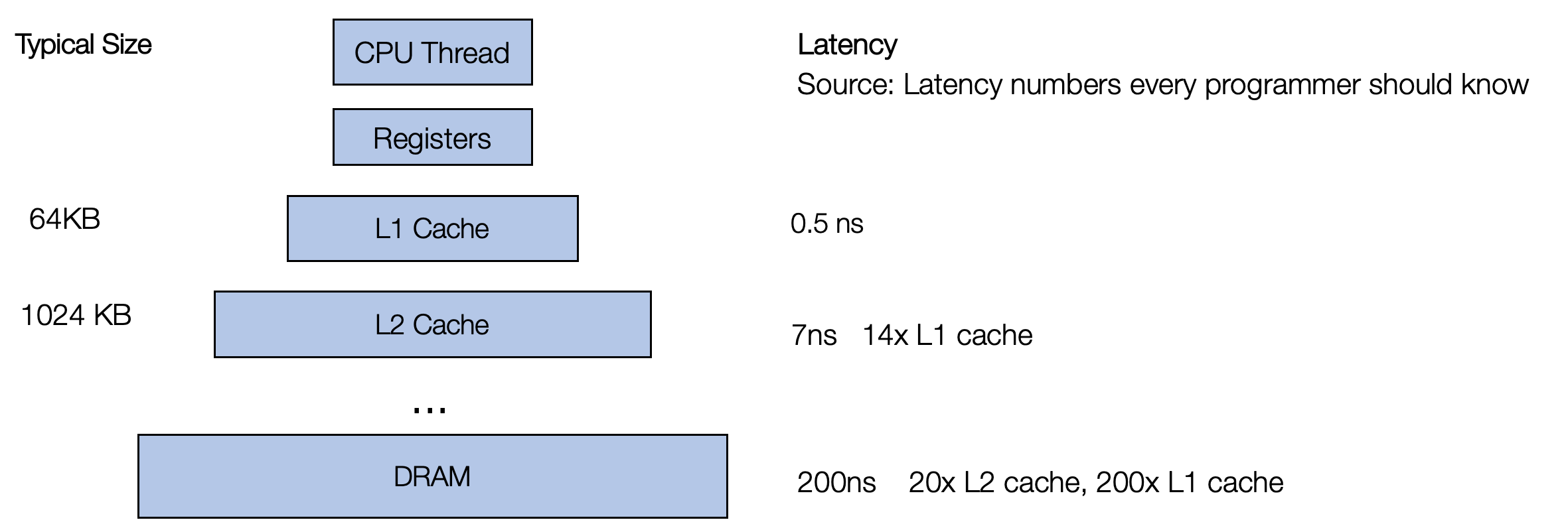
To see why different loop variants result in different performances, we
need to review the fact that it is not uniformly fast to access any
piece of memory in A and B. Modern CPU comes with multiple
levels of caches, where data needs to be fetched into the cache before
the CPU can access it.
Importantly, it is much faster to access the data already in the cache. One strategy that CPU takes is to fetch data closer to each other. When we read one element in the memory, it will attempt to fetch the elements close by (formally known as cache-line) to the cache. So when you read the next element, it is already in the cache. As a result, code with continuous memory access is usually faster than code that randomly accesses different parts of the memory.
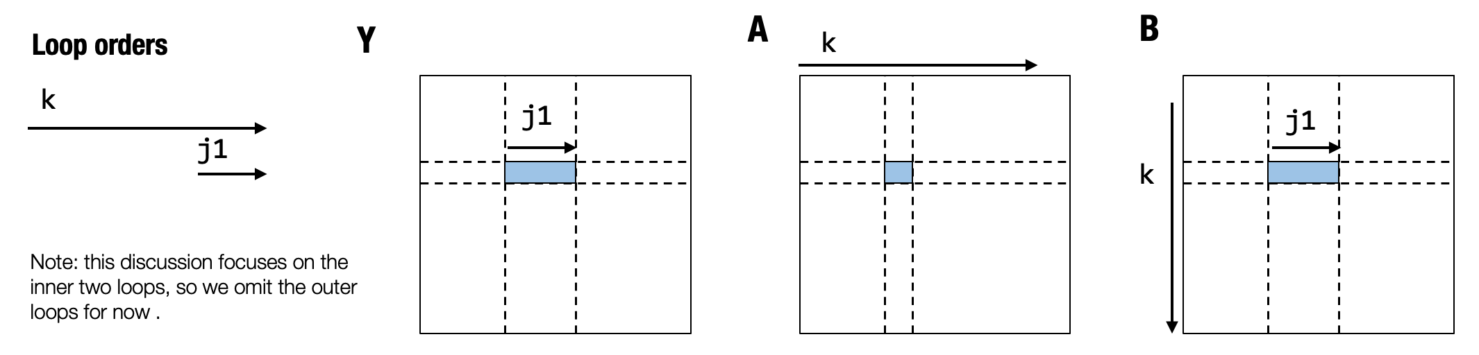
Now let us look at the above visualization of iterations and analyze
what is going on. In this analysis, let us focus on two inner-most
loops: k and j1. The highlighted cover shows the corresponding
region in Y, A and B that the iteration touches when we
iterate over j1 for one specific instance of k.
We can find that the j1 iteration produces continuous access to
elements of B. Specifically, it means the values we read when
j1=0 and j1=1 are next to each other. This enables better cache
access behavior. In addition, we bring the computation of C closer to
Y, enabling better caching behavior.
Our current example is mainly to demonstrate that different variants of code can lead to different performances. More transformation steps can help us to get to even better performance, which we will cover in future chapters. The main goal of this exercise is first to get us the tool of program transformations and first taste of what is possible through transformations.
2.4.5.1. Exercise
As an exercise, try different j_factor choices and see how they
affect the code’s performance.
def transform(mod, jfactor):
    sch = tvm.tir.Schedule(mod)
    block_Y = sch.get_block("Y", func_name="mm_relu")
    i, j, k = sch.get_loops(block_Y)
    j0, j1 = sch.split(j, factors=[None, jfactor])
    sch.reorder(j0, k, j1)
    block_C = sch.get_block("C", "mm_relu")
    sch.reverse_compute_at(block_C, j0)
    return sch.mod

mod_transformed = transform(MyModule, jfactor=8)

rt_lib_transformed = tvm.build(mod_transformed, "llvm")
f_timer_transformed = rt_lib_transformed.time_evaluator("mm_relu", tvm.cpu())
print("Time cost of transformed mod_transformed %g sec" % f_timer_transformed(a_nd, b_nd, c_nd).mean)
# display the code below
IPython.display.Code(mod_transformed.script(), language="python")
Time cost of transformed mod_transformed 0.000380994 sec
# from tvm.script import ir as I
# from tvm.script import tir as T

@I.ir_module
class Module:
    @T.prim_func
    def mm_relu(A: T.Buffer((128, 128), "float32"), B: T.Buffer((128, 128), "float32"), C: T.Buffer((128, 128), "float32")):
        T.func_attr({"tir.noalias": T.bool(True)})
        # with T.block("root"):
        Y = T.alloc_buffer((128, 128))
        for i, j_0 in T.grid(128, 16):
            for k, j_1 in T.grid(128, 8):
                with T.block("Y"):
                    vi = T.axis.spatial(128, i)
                    vj = T.axis.spatial(128, j_0 * 8 + j_1)
                    vk = T.axis.reduce(128, k)
                    T.reads(A[vi, vk], B[vk, vj])
                    T.writes(Y[vi, vj])
                    with T.init():
                        Y[vi, vj] = T.float32(0.0)
                    Y[vi, vj] = Y[vi, vj] + A[vi, vk] * B[vk, vj]
            for ax0 in range(8):
                with T.block("C"):
                    vi = T.axis.spatial(128, i)
                    vj = T.axis.spatial(128, j_0 * 8 + ax0)
                    T.reads(Y[vi, vj])
                    T.writes(C[vi, vj])
                    C[vi, vj] = T.max(Y[vi, vj], T.float32(0.0))
2.4.6. Ways to Create and Interact with TensorIR
In the last sections, we learned about TensorIR abstraction and ways to transform things. TensorIR comes with an additional construct named block that helps us analyze and perform code transformations. One natural question we might ask: what are common ways to create and interact with TensorIR functions?
2.4.6.1. Create TensorIR via TVMScript
The first way to get a TensorIR function is to write a function in
TVMScript directly, and this is also the approach we use in the last
sections. TVMScript also allows us to skip certain parts of information
when necessary. For example, T.axis.remap enables us to shorten the
iterator size annotations.
TVMScript is also a useful way to inspect the tensor functions in the middle of transformations. In some instances, it might be helpful to print out the script, do some manual editing, then feed it back to the MLC process just to debug and try out possible transformation (manually), then bake it into the MLC process.
2.4.6.2. Generate TensorIR code using Tensor Expression
In many cases, our development forms are higher-level abstractions that are not at the loop level. So another common way to obtain TensorIR is programmatically generating relevant code.
Tensor expression (te) is a domain-specific language that describes a sequence of computations via an expression-like API.
from tvm import te

A = te.placeholder((128, 128), "float32", name="A")
B = te.placeholder((128, 128), "float32", name="B")
k = te.reduce_axis((0, 128), "k")
Y = te.compute((128, 128), lambda i, j: te.sum(A[i, k] * B[k, j], axis=k), name="Y")
C = te.compute((128, 128), lambda i, j: te.max(Y[i, j], 0), name="C")
Here te.compute takes the signature
te.compute(output_shape, fcompute). And the fcompute function
describes how we want to compute the value of each element Y[i, j]
for a given index.
lambda i, j: te.sum(A[i, k] * B[k, j], axis=k)
The above lambda expression describes the computation \(Y_{ij} = \sum_k A_{ik} B_{kj}\). After describing the computation, we can create a TensorIR function by passing the relevant parameter we are interested in. In this particular case, we want to create a function with two input parameters (A, B) and one output parameter (C).
te_func = te.create_prim_func([A, B, C]).with_attr({"global_symbol": "mm_relu"})
MyModuleFromTE = tvm.IRModule({"mm_relu": te_func})
IPython.display.Code(MyModuleFromTE.script(), language="python")
# from tvm.script import ir as I
# from tvm.script import tir as T

@I.ir_module
class Module:
    @T.prim_func
    def mm_relu(A: T.Buffer((128, 128), "float32"), B: T.Buffer((128, 128), "float32"), C: T.Buffer((128, 128), "float32")):
        T.func_attr({"tir.noalias": T.bool(True)})
        # with T.block("root"):
        Y = T.alloc_buffer((128, 128))
        for i, j, k in T.grid(128, 128, 128):
            with T.block("Y"):
                v_i, v_j, v_k = T.axis.remap("SSR", [i, j, k])
                T.reads(A[v_i, v_k], B[v_k, v_j])
                T.writes(Y[v_i, v_j])
                with T.init():
                    Y[v_i, v_j] = T.float32(0.0)
                Y[v_i, v_j] = Y[v_i, v_j] + A[v_i, v_k] * B[v_k, v_j]
        for i, j in T.grid(128, 128):
            with T.block("C"):
                v_i, v_j = T.axis.remap("SS", [i, j])
                T.reads(Y[v_i, v_j])
                T.writes(C[v_i, v_j])
                C[v_i, v_j] = T.max(Y[v_i, v_j], T.float32(0.0))
The tensor expression API provides a helpful tool to generate TensorIR functions for a given higher-level input.
2.4.7. TensorIR Functions as Results of Transformations
In practice, we also get TensorIR functions as results of
transformations. This happens when we start with two primitive tensor
functions (mm and relu), then apply a programmatic transformation to
“fuse” them into a single primitive tensor function, mm_relu. We
will cover the details in future chapters.
2.4.8. Discussions
In this section, let us review what we learned so far. We learned that a common MLC process follows a sequence of program transformations. It is interesting to compare the TensorIR transformation process to the low-level numpy reference development process.
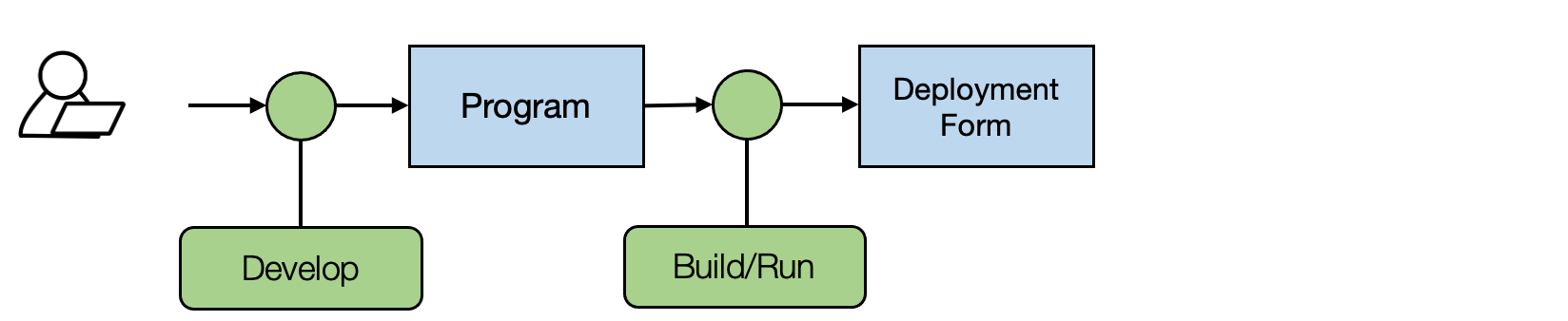
The above figure shows the standard development process. We need to repeat the process of developing different program variants and then (build if it is a compiled language) run them on the platform of interest.
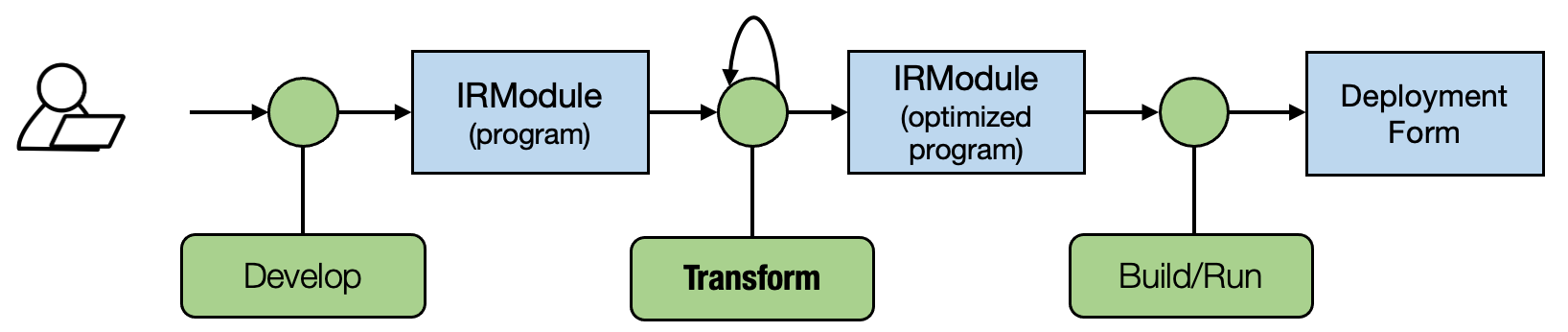
The key difference in an MLC process(shown in the figure below) is the programmatic transformations among the IRModule (programs). So we can not only come up with program variants through development (either by manually writing the code or generating the code), but also can obtain variants by transforming the tensor programs.
Transformation is a very powerful tool that helps us simplify development costs and introduce more automation to the process. This section covered a specific perspective on primitive tensor functions via TensorIR, and we will cover more perspectives in the future.
Notably, direct code development and transformations are equally important in practice: We can still leverage a lot of domain expertise to develop and optimize part of the programs and then combine that with transformation-based approaches. We will talk about how to combine the two practices in future chapters.
2.4.9. Summary
TensorIR abstraction
Contains common elements such as loops, multi-dimensional buffers
Introduced a new construct Block that encapsulates the loop computation requirements.
Can be constructed in python AST(via TVMScript)
We can use transformations to create different variants of TensorIR.
Common MLC flow: develop, transform, build.